walker's code blog

coder, reader

《Deep Learning with Python》笔记[3]

Fundamentals of machine learning

  • Supervised learning
    • binary classification
    • multiclass classificaiton
    • scalar regression
    • vector regression(比如bounding-box)
    • Sequence generation (摘要,翻译...)
    • Syntax tree prediction
    • Object detection (一般bounding-box的坐标仍然是回归出来的)
    • Image segmentation
  • Unsupervised learing
    • 是数据分析的基础,在监督学习前也常常需要用无监督学习来更好地“理解”数据集
    • 主要有降维(Dimensionality reduction)和聚类(clustering)
  • Self-supervised learning
    • 其实还是监督学习,因为它仍需要与某个target做比较
    • 往往半监督(自监督)学习仍然有小量有标签数据集,在此基础上训练的不完善的model用来对无标签的数据进行打标,循环中对无标签数据打标的可靠度就越来越高,这样总体数据集的可靠度也越来越高了。有点像生成对抗网络里生成器和辨别器一同在训练过程中完善。
    • autoencoders
  • Reinforcement learning
    • an agent receives information about its environment and learns to choose actions that will maximize some reward.
    • 可以用训练狗来理解
    • 工业界的应用除了游戏就是机器人了

Data preprocessing

  • vectorization
  • normalization (small, homogenous)
  • handling missing values
    1. 除非0有特别的含义,不然一般可以对缺失值补0
    2. 你不能保证测试集没有缺失值,如果训练集没看到过缺失值,那么将不会学到忽略缺失值
      • 复制一些训练数据并且随机drop掉一些特征
  • feature extraction
    • making a problem easier by expressing it in a simpler way. It usually requires understanding the problem in depth.
    • Before deep learning, feature engineering used to be critical, because classical shallow algorithms didn’t have hypothesis spaces rich enough to learn useful features by themselves. (又见假设空间)
    • 但是好的特征仍然能让你在处理问题上更优雅、更省资源,也能减小对数据集规模的依赖。

Overfitting and underfitting

  • Machine learning is the tension between optimization and generalization.
  • optimization要求你在训练过的数据集上能达到最好的效果
  • generalization则希望你在没见过的数据上有好的效果
  • 如果训练集上loss小,测试集上也小,说明还有优化(optimize)的余地 -> underfitting看loss
    • just keep training
  • 如果验证集上generalization stop improving(泛化不再进步,一般看衡量指标,比如准确率) -> overfitting

解决overfitting的思路:

  • the best solution is get more trainging data
  • the simple way is to reduce the size of the model
    • 模型容量(capacity)足够大,就足够容易记住input和target的映射,没推理什么事了
  • add constraints -> weight regularization
  • add dropout

Regularization

Occam’s razor

given two explanations for something, the explanation most likely to be correct is the simplest one—the one that makes fewer assumptions.

即为传说中如无必要,勿增实体奥卡姆剃刀原理,这是在艺术创作领域的翻译,我们这里还是直译的好,即能解释一件事的各种理解中,越简单的,假设条件越少的,往往是最正确的,引申到机器学习,就是如何定义一个simple model

A simple model in this context is:

  • a model where the distribution of parameter values has less entropy
  • or a model with fewer parameters

实操就是,就是迫使选择那些值比较小的weights,which makes the distribution of weight values more regular. This is called weight regularization。这个解释是我目前看到的最regularization这个名字最好的解释,“正则化”三个字都认识,根本没人知道这三个字是什么意思,翻译了跟没番一样,而使分布更“常规化,正规化”,好像更有解释性。

别的教材里还会告诉你这里是对大的权重的惩罚(设计损失函数加上自身权重后,权重越大,loss也就越大,这就是对大权重的惩罚)

  • L1 regularization—The cost added is proportional to the absolute value of the weight coefficients (the L1 norm of the weights).
  • L2 regularization—The cost added is proportional to the square of the value of the weight coefficients (the L2 norm of the weights).

L2 regularization is also called weight decayin the context of neural networks. Don’t let the different name confuse you: weight decay is mathematically the same as L2 regularization.

只需要在训练时添加正则化

Dropout

randomly dropping out (setting to zero) a number of output features of the layer during training.

dropout的作者Geoff Hinton解释dropout的灵感来源于银行办事出纳的不停更换和移动的防欺诈机制,可能认为一次欺诈的成功实施需要员工的配合,所以就尽量降低这种配合的可能性。于是他为了防止神经元也能聚在一起”密谋”,尝试随机去掉一些神经元。以及对输出添加噪声,让模型更难记住某些patten。

The universal workflow of machine learning

  1. Defining the problem and assembling a dataset
    • What will your input data be?
    • What are you trying to predict?
    • What type of problem are you facing?
    • You hypothesize that your outputs can be predicted given your inputs.
    • You hypothesize that your available data is sufficiently informative to learn the relationship between inputs and outputs.
    • Just because you’ve assembled exam- ples of inputs X and targets Y doesn’t mean X contains enough information to predict Y.
  2. Choosing a measure of success
    • accuracy? Precision and recall? Customer-retention rate?
    • balanced-classification problems,
      • accuracy and area under the receiver operating characteristic curve (ROC AUC)
    • class-imbalanced problems
      • precision and recall.
    • ranking problems or multilabel classification
      • mean average precision
    • ...
  3. Deciding on an evaluation protocol
    • Maintaining a hold-out validation set—The way to go when you have plenty of data
    • Doing K-fold cross-validation—The right choice when you have too few samples for hold-out validation to be reliable
    • Doing iterated K-fold validation—For performing highly accurate model evaluation when little data is available
  4. Preparing your data
    • tensor化,向量化,归一化等
    • may do some feature engineering
  5. Developing a model that does better than a baseline
    • baseline:
      • 基本上是用纯随机(比如手写数字识别,随机猜测为10%),和纯相关性推理(比如用前几天的温度预测今天的温度,因为温度变化是连续的),不用任何机器学习做出baseline
    • model:
      • Last-layer activation
        • sigmoid, relu系列, 等等
      • Loss function
        • 直接的预测值真值的差,如MSE
        • 度量代理,如crossentropy是ROC AUC的proxy metric
    • Optimization configuration
      • What optimizer will you use? What will its learning rate be? In most cases, it’s safe to go with rmsprop and its default learning rate.
    • Scaling up: developing a model that overfits
      • 通过增加layers, 增加capacity,增加training epoch来加速overfitting,从而再通过减模型和加约束等优化
    • Regularizing your model and tuning your hyperparameters
      • Add dropout.
      • Try different architectures: add or remove layers.
      • Add L1 and/or L2 regularization.
      • Try different hyperparameters (such as the number of units per layer or the learning rate of the optimizer) to find the optimal configuration.
      • Optionally, iterate on feature engineering: add new features, or remove features that don’t seem to be informative.
Problem type Last-layer activation Loss function
Binary classification sigmoid binary_crossentropy
Multiclass, single-label classification softmax categorical_crossentropy
Multiclass, multilabel classification sigmoid binary_crossentropy
Regression to arbitrary values None mse
Regression to values between 0 and 1 sigmoi mse or binary_crossentropy

《Deep Learning with Python》笔记[2]

Getting started with neural networks

Anatomy of a neural network

  • Layers, which are combined into a network (or model)
    • layers: 常见的比如卷积层,池化层,全连接层等
    • models: layers构成的网络,或多个layers构成的模块(用模块组成网络)
      • Two-branch networks
      • Multihead networks
      • Inception blocks, residual blocks etc.
    • The topology of a network defines a hypothesis space
    • 本书反复强调的就是这个hypothesis space,一定要理解这个思维:
      • By choosing a network topology, you constrain your space of possibilities (hypothesis space) to a specific series of tensor operations, mapping input data to output data.(network的选择约束了tensor变换的步骤)
      • 所以如果选择了不好的network,可能导致你在错误的hyposhesis space里搜索,以致于效果不好。
  • The input data and corresponding targets
  • The loss function (objective function), which defines the feedback signal used for learning
    • The quantity that will be minimized during training.
    • It represents a measure of success for the task at hand.
    • 多头网络有多个loss function,但基于gradient-descent的网络只允许有一个标量的loss,因此需要把它合并起来(相加,平均...)
  • The optimizer, which determines how learning proceeds
    • Determines how the network will be updated based on the loss function.
    • It implements a specific variant of stochastic gradient descent (SGD).

Classifying movie reviews: a binary classification example

一个二元分类的例子

情感分析/情绪判断,数据源是IMDB的影评数据.

理解hidden的维度

how much freedom you’re allowing the network to have when learning internal representations. 即学习表示(别的地方通常叫提取特征)的自由度。

目前提出了架构网络的时候的两个问题:

  1. 多少个隐层
  2. 隐层需要多少个神经元(即维度)

后面的章节会介绍一些原则。

激活函数

李宏毅的课程里,从用整流函数来逼近非线性方程的方式来引入激活函数,也就是说在李宏毅的课程里,激活函数是,推出来的公式是,当然一般的教材都不是这个角度,都是有了线性方程,再去告诉你,这样还不够,需要一个activation

本书也一样,告诉你,如果只有wX+b,那么只有线性变换,这样会导致对hypothesis space的极大的限制,为了扩展它的空间,就引入了非线性的后续处理。总之,都是在自己的逻辑体系内的。本书的逻辑体系就是hypothesis space,你想要有解,就是在这个空间里。

网络结构

from keras import models
from keras import layers
model = models.Sequential()
model.add(layers.Dense(16, activation='relu', input_shape=(10000,)))
model.add(layers.Dense(16, activation='relu'))
model.add(layers.Dense(1, activation='sigmoid'))

entropy

Crossentropy is a quantity from the field of Information Theory(信息论) that measures the distance between probability distributions。

in this case, between the ground-truth distribution and your predictions.

keras风格的训练

其实就是模仿了scikit learn的风格。对快速实验非常友好,缺点就是封装过于严重,不利于调试,但这其实不是问题,谁也不会只用keras。

# 演示用类名和字符串分别做参数的方式
model.compile(optimizer='rmsprop',
            loss='binary_crossentropy',
            metrics=['accuracy'])

from keras import optimizers
model.compile(optimizer=optimizers.RMSprop(lr=0.001),
            loss='binary_crossentropy',
            metrics=['accuracy'])

from keras import losses
from keras import metrics
model.compile(optimizer=optimizers.RMSprop(lr=0.001),
            loss=losses.binary_crossentropy,
            metrics=[metrics.binary_accuracy])

model.compile(optimizer='rmsprop',
              loss='binary_crossentropy',
              metrics=['acc'])

# train
history = model.fit(partial_x_train,
                    partial_y_train,
                    epochs=20,
                    batch_size=512,
                    validation_data=(x_val, y_val))

后续优化,就是对比train和validate阶段的loss和accuracy,找到overfit的节点(比如是第N轮),然后重新训练到第N轮(或者直接用第N轮生成的模型,如果有),用这个模型来预测没有人工标注的数据。

核心就是要训练到明显的overfit为止。这是第一个例子的内容,所以是告诉你怎么用这个简单的网络来进行预测,而不是立即着眼怎么去解决overfit.

第一个小结

  1. 数据需要预处理成tensor, 了解几种tensor化,或vector化的方式
  2. 堆叠全连接网络(Dense),以及activation,就能解决很多分类问题
  3. 二元分类的问题通常在Dense后接一个sigmoid函数
  4. 引入二元交叉熵(BCE)作为二元分类问题的loss
  5. 用了rmsprop优化器,暂时没有过多介绍。这些优化器都是为了解决能不能找到局部极值而进行的努力,具体可看上一篇李宏毅的笔记
  6. 使用overfit之前的那一个模型来做预测

Classifying newswires: a multiclass classification example

这次用路透社的新闻来做多分类的例子,给每篇新闻标记类别。

预处理,一些要点:

  1. 不会采用所有的词汇,所以预处理时,根据词频,只选了前1000个词
  2. 用索引来实现文字-数字的对应
  3. 用one-hot来实现数字-向量的对应
  4. 理解什么是序列(其实就是一句话)
  5. 所以句子有长有短,为了矩阵的批量计算(即多个句子同时处理),需要“对齐”(补0和截断)
  6. 理解稠密矩阵(word-embedding)与稀疏矩阵(one-hot)的区别(这里没有讲,用的是one-hot)

网络和训练

  1. 网络结构不变,每层的神经元为(64, 64, 46)
  2. 前面增加了神经元,16个特征对语言来说应该是不够的)
  3. 最后一层由1变成了46,因为二元的输出只需要一个数字,而多元输出是用one-hot表示的向量,最有可能的类别在这个向量里拥有最大的值。

4。 损失函数为categorial_crossentropy,这在别的教材里应该就是普通的CE.

新知识

  1. 介绍了一种不用one-hot而直接用数字表示真值的方法,但是没有改变网络结构(即最后一层仍然输出46维,而不是因为你用了一个标量而只输出一维。
    • 看来它仅仅就是一个语法糖(loss函数选择sparse_categorial_crossentropy就行了)
  2. 尝试把第2层由64改为4,变成bottleneck,演示你有46维的数据要输出的话,前面的层数或少会造成信息压缩过于严重以致于丢失特征。

Predicting house prices: a regression example

这里用了预测房价的Boston Hosing Price数据集。

与吴恩达的课程一样,也恰好是在这个例子里引入了对input的normalize,理由也仅仅是简单的把量纲拉平。现在我们应该还知道Normalize还能让数据在进入激活函数前,把值限定在激活函数的梯度敏感区。

此外,一个知识点就是你对训练集进行Normalize用的均值和标准差,是直接用在测试集上的,而不是各计算各的,可以理解为保持训练集的“分布”。

这也是scikit learnfit_tranform和直接用transform的原因。

  1. 对scalar进行预测是不需要进行激活(即无需把输出压缩到和为1的概率空间)
  2. loss也直观很多,就是predict与target的差(取平方,除2,除批量等都是辅助),预测与直值的差才是核心。

《Deep Learning with Python》笔记[1]

本来是打算趁这个时间好好看看花书的,前几章看下来确实觉得获益匪浅,但看下去就发现跟不上了,特别是抱着急功近利的心态的话,目前也沉不下去真的一节节吃透地往下看。这类书终归不是入门教材,是需要你有过一定的积累后再回过头来看的。

于是想到了《Deep Learning with Python》,忘记这本书怎么来的了,但是在别的地方看到了有人推荐,说是Keras的作者写的非常好的一本入门书,翻了前面几十页后发现居然跟进去了,不该讲的地方没讲比如数学细节,而且思路也极其统一,从头贯穿到尾(比如representations, latent space, hypothesis space),我觉得很受用。

三百多页全英文,居然也没查几个单词就这么看完了,以前看文档最多十来页,也算一个突破了,可见其实还是一个耐心的问题。

看完后书上做了很多笔记,于是顺着笔记读了第二遍,顺便就把笔记给电子化了。不是教程,不是导读。

Fundamentals of deep learning

核心思想: learng useful representations of input data

what’s a representation?

At its core, it’s a different way to look at data—to represent or encode data.

简单回顾深度学习之于人工智能的历史,每本书都会写,但每本书里都有作者自己的侧重:

  • Artificial intelligence
  • Machine learning
    • Machine learning is tightly related to mathematical statistics, but it differs from statistics in several important ways.
      • machine learning tends to deal with large, complex datasets (such as a dataset of millions of images, each consisting of tens of thousands of pixels)
      • classical statistical analysis such as Bayesian analysis would be impractical(不切实际的).
      • It’s a hands-on discipline in which ideas are proven empirically more often than theoretically.(工程/实践大于理论)
    • 是一种meaningfully transform data
      • Machine-learning models are all about finding appropriate representations for their input data—transformations of the data that make it more amenable to the task at hand, such as a classification task.
      • 寻找更有代表性的representation, 通过:(coordinate change, linear projections, tranlsations, nonlinear operations)
      • 只会在hypothesis space里寻找
      • 以某种反馈为信号作为优化指导
  • Deep learning
    • Machine Learing的子集,一种新的learning representation的新方法
    • 虽然叫神经网络(neural network),但它既非neural,也不是network,更合理的名字:
      • layered representations learning and hierarchical representations learning.
    • 相对少的层数的实现叫shallow learning

Before deep learning

  • Probabilistic modeling
    • the earliest forms of machine learning,
    • still widely used to this day.
      • One of the best-known algorithms in this category

is the Naive Bayes algorithm(朴素贝叶斯) * 条件概率,把规则理解为“条件”,判断概率,比如垃圾邮件。 * A closely related model is the logistic regression

  • Early neural networks
    • in the mid-1980s, multiple people independently rediscovered the Backpropagation algorithm
    • The first successful practical application of neural nets came in 1989 from Bell Labs -> LeNet
  • Kernel methods
    • Kernel methods are a group of classification algorithms(核方法是一组分类算法)
      • the best known of which is the support vector machine (SVM).
      • SVMs aim at solving classification problems by finding good decision boundaries between two sets of points belonging to two different categories.
        1. 先把数据映射到高维,decision boundary表示为hyperplane
        2. 最大化每个类别里离hyperplane最近的点到hyperplane的距离:maximizing the margin
      • The technique of mapping data to a high-dimensional representation 非常消耗计算资源,实际使用的是核函数(kernel function):
        • 不把每个点转换到高维,而只是计算每两个点在高维中的距离
        • 核函数是手工设计的,不是学习的
      • SVM在分类问题上是经典方案,但难以扩展到大型数据集上
      • 对于perceptual problems(感知类的问题)如图像分类效果也不好
        • 它是一个shallow method
        • 需要事先手动提取有用特征(feature enginerring)-> difficult and brittle(脆弱的)
  • Decision trees, random forests, and gradient boosting machines
    • Random Forest
      • you could say that they’re almost always the second-best algorithm for any shallow machine-learning task.
    • gradient boosting machines (1st):
      • a way to improve any machine-learning model by iteratively training new models that specialize in addressing the weak points of the previous models.

What makes deep learning different

it completely automates what used to be the most crucial step in a machine-learning workflow: feature engineering. 有人认为这叫穷举,思路上有点像,至少得到特征的过程不是靠观察和分析。

feature engineering

manually engineer good layers of representations for their data

几大排序算法python实现

冒泡排序

冒泡排序基础原理是每一轮都让最大的值移到最右边,一句话就够了。

如果想小优化一下,可以在每一轮过后都把最后一个(已经是最大的值)排除出去,这种我把它称之为“压缩边界“,在下面的几种排序算法里都有反复提及。而且之所以说优化,就是不做也行,如果只是想演示算法核心思想的话。

def bubble_sort(arr):
    for i in range(1, len(arr)):
        for j in range(len(arr)-i):
            if arr[j] > arr[j+1]:
                arr[j], arr[j+1] = arr[j+1], arr[j]
    return arr
bubble_sort([0, 2, 1, 3, 5, 1, 1])

ouput:

[0, 1, 1, 1, 2, 3, 5]

快速排序

选出一个合适的(或任意的)中值(pivot),把比它大的和小的分列到两边,再对两边进行上述分类的递归操作。实际操作中往往会选定了pivot后,从右往左搜小数,从左往右搜大数,以规避pivot本身过大或过小时,如果选定的方向不对,可能每一次都需要把整个数组几乎遍历完才找到合适的数的情况。

again,这只是优化,如果不考虑这些,那么核心思想是非常简单的:

def q_sort(arr):
    if len(arr) <= 1:
        return arr
    pivot = arr.pop()
    left  = [item for item in arr if item <= pivot]
    right = [item for item in arr if item > pivot]
    return q_sort(left) + [pivot] + q_sort(right)

这个不但实现了(中值+两侧+递归)的思路+没有任何优化,效果已经出奇的好了!

但网上演示的都是下面这种花活,从两侧来压缩备选区域(压缩的意思是排好了的区域就不要管了),下面列了个表格来演示过程,看大家是不是能轻松看懂快排的两个核心机制:标红位,和边界压缩。说明如下:

  • 任意写个数组[6,7,3,2,14,9],任取一个数为pivot,就第1个吧(6),
  • 左箭头表示从右往左找第一个小于pivot的值,右箭头表示从左往右找第一个大于pivot的值
  • 红色代表标红位,废位,即当前位找到本轮符合要求的值,但挪到两侧去了,$\color{red}{下一轮的符合条件的值应该放入这个标红位里}$
  • 括号里的表示是这一轮该位置赋的新值,它来自于标红位,同时,括号的位置也就是上一轮的标红位
  • 划掉的表示已经压缩了左右边界,下一轮就不要在这些数里面选了(为了视觉简洁,标红位就不划了)

$$ \require{cancel} \begin{array}{c|cccccc|l} index&0&1&2&3&4&5&\\ \hline array&\color{red}6&7&3&2&14&9\\ \underleftarrow{\small找小数}&\cancel{(2)}&7&3&\color{red}2&\cancel{14}&\cancel{9}&找到2,放到索引0\\ \underrightarrow{\small找大数}&\cancel{2}&\color{red}7&3&(7)&\cancel{14}&\cancel{9}&找到7,放到索引3\\ \underleftarrow{\small找小数}&\cancel{2}&(3)&\color{red}3&\cancel{7}&\cancel{14}&\cancel{9}&找到3,放到索引2\\ &2&3&(6)&7&14&9&(1,2)索引间已没有大于6的数,排序完成,回填6 \end{array} $$

  1. 注意第1次从右往左找比6小的数时,找到2,右边的14,9就可以全部划掉了,因为我永远是在用6在左右查找,这一次pass了,后面永远会pass
  • 这样边界压缩得非常快,这就是称之为“快速”排序的原因吧?
  1. 目前只完成一次分割(即按6为标识切分左右),接下来用同样的逻辑递归6左边的[2]和右边的[7,14,9]排序即可
  • 所以快排就3个部分,一个主体,执行一次分割,然后对分割后的两个数组分别递归回去,这样代码怎么写也出来了:
def q_sort(array, start, end):
    # (left, right)用来保存不断缩小的查找数组索引界限
    #  我上面模拟的过程里,就是划掉的数字的左右边界
    left, right = start, end
    index = start
    pivot = array[start]

    while left < right:
        # 从右往左选小于pivot的数
        matched = False # 标识这一轮有没有找到合适的数(如果没找到其实说明排序已经完成)
        for i in reversed(range(left+1, right+1)): # 去头,含尾, 反序
            if array[i] <= pivot:
                array[index] = array[i]
                right = i  # 从右到左比到第i个才有比pivot小的数,那么i右侧全大于pivot,下次可以缩小范围了
                index = i
                matched = True
                break
        if not matched:
            break  # 右侧没有找到更小的数,说明剩余数组全是大数,已经排完了

        left += 1 # 找到了填入新数后就顺移一位
        matched = False
        # 从左往右选大于pivot的数
        for i in range(left, right): # 有头无尾
            if array[i] > pivot:
                array[index] = array[i]
                left = i # 此时i左侧也没有比pivot大的数,下次再找也可以忽略了,也标记下缩小范围
                index = i
                matched = True
                break;
        if not matched:
            break
        right -= 1
    array[index] = pivot # 把标红位设为pivot

    # 开始递归处理左右切片
    if start < index-1:
        q_sort(array, start, index-1)
    if end > index+1:
        q_sort(array, index+1, end)

    return array

arr = [0, 2, 1, 3, 5, 1, 1]
# 我封装时为了兼容递归,要人为传入start, end,进入函数时自行计算一下好了
q_sort(arr, 0, len(arr)-1)

output

[0, 1, 1, 1, 2, 3, 5]

堆排序

  1. 其实就是把数字摆成二叉树,知道二叉树是啥就行,或者看下面的动图
  2. 每当一个数字排入堆中的时候,都与父节点比一下大小,如果大于父节点,则与父节点交换位置
  • 不与兄弟节点比较,即兄弟节点之间暂不排序
  1. 交换到父节点后再跟当前位置的父节点比较,如此往复,至到根节点(递归警告
  2. 一轮摆完后,最大的数肯定已经上浮到根节点了,把它与最末的一个数字调换位置(这个数字是一个相对小,但不一定是最小的),然后把最大的这个数从堆里移除(已经确认是最大的,位置也就确认了,不再参与比较)
  3. 实现的时候,因为有“找父/子节点比大小”这样的逻辑,显然可以直接用上二叉树的性质,不要自己去观察或归纳了。

动图比较长,耐心看下:

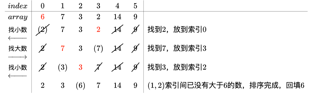
在实现每一轮的遍历数字较大的那个子节点并交换数字的过程中,我之前用的是递归,在小数据量顺利通过,但上万条数据时碰到了RecursionError: maximum recursion depth exceeded in comparison, 查询本机迭代大小设置为1000,但设到几十万就不起作用了(虽然不报错),于是改成了while循环,代码几乎没变,但是秒过了。
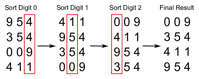
递归只是让代码看起来简洁而牛逼,并没有创造什么新的东西,while能行那就算过了吧。

但是代码开始dirty了起来,大量的代码在控制边界和描述场景,显然有些条件可能是冗余的,我没有很好地合并这些边界和条件导致if太多,这是个不好的演示,但三个核心函数还是阐释了这种算法的思路:

  • 摆成树(堆)
  • 从leaf到root冒泡 (child去比parent)
  • 从root到leaf冒泡 (parent去比child)
# helper
get_parent_index = lambda i : max((i - 1) // 2, 0)
get_child_index  = lambda i : 2 * i + 1

def heap_sort(arr):
    heapify(arr)                    # 初排
    siftDown(arr, 0, len(arr)-1)    # 整理
    return arr

def heapify(arr):
    index = 1
    while index < len(arr):
        p_index = get_parent_index(index)
        parent  = arr[p_index]
        child   = arr[index]
        if child > parent:
            arr[p_index], arr[index] = arr[index], arr[p_index]
            siftUp(arr, p_index)
        index += 1
    return arr

def siftUp(arr, c_index):
    p_index = get_parent_index(c_index)
    parent  = arr[p_index]
    leaf    = arr[c_index]
    if parent < leaf:
        arr[p_index], arr[c_index] = arr[c_index], arr[p_index]
    if p_index > 0:
        siftUp(arr, p_index)

def siftDown(arr, start, end):
    '''
    1. 交换首尾两个数,这样尾数就变成了最大
    2. 跟两个子节点中较大的比较,并迭代,递归下去
    '''
    while start < end:
        if start == 0:
            arr[0], arr[end] = arr[end], arr[0]
        left_i  = get_child_index(start)
        if left_i >= end: 
            # 子结点是end,就不要比了,把当前节点设为新end
            start = 0
            end -= 1
            continue
        else:
            right_i = left_i + 1
            index = left_i
            if right_i < end:
                # 右边没有到end的话,取出值比大小
                # 并且把下一轮的start设为选中的子节点
                index = left_i if arr[left_i] > arr[right_i] else right_i
            parent  = arr[start]
            if parent < arr[index]:
                arr[start], arr[index] = arr[index], arr[start]
        # 如果左叶子已经被标记为end  (已提前return)
        # 如果右边叶子被标记为end
        # 如果下一个索引被标记为end
        # 都表示本轮遍历已经到底, end往前移一位即可
        if right_i >= end or (end - right_i) == 1:
            start = 0 # 用start=0表示需要进行一次首尾替换再从头到尾移动一次
            end -= 1
        else:
            # 否则进入下一个循环
            # 起点就是用来跟父级做比较的索引
            # 终点不变
            start = index

if __name__ == "__main__":
    import numpy as np
    import time
#     np.random.seed(7)
#     length = 20000
#     arr = list(np.random.randint(0, length*5, size=(length,)))
    arr = list("65318724")
    start = time.time()
    s = heap_sort(arr)
    print(time.time()-start, '\n', s[:100])

output

4.696846008300781e-05 
 ['1', '2', '3', '4', '5', '6', '7', '8']

归并排序

这次先看图吧,看你能总结出啥:

  1. 第一步是把数组打散后两两排序,实现每一组(2个元素)是排好序的
  2. 第二步仍然是两两排序,但是把前面排序好的每两个组成一个组:
  • 这样每组就有2个数了,但组数就减半了
  • 每一组拿出当前最前面的数出来比较,每次挑1个最小的,移出来
  • 剩下的组里数字有多有少,仍然比较组里面排最前的那个(因为每组已经从小到大排好了,最前面那个就是组里最小的)
  • 所以代码里能跟踪两个组里当前的“最前的索引”是多少就行了
  1. 继续合并,单从理论上你也能发现,每组的数字个数会越来越多,组数却越来越少, 显然,最终会归并成一个组,而且已经是排好序了的。

这就是归并名字的由来。后面还有一种希尔算法,正好是它的相反,即打得越来越散,散成每组只有一个元素的时候,排序也排好了,看到那一节的时候注意对比。

import math
def merge_sort(arr):
    '''
    每一轮比较的时候是把选中的元素填到另一个数组里
    为了减少内存消耗,就循环用两个数组
    我们用交替设置i和j为0和1来实现这个逻辑
    '''
    start    = 0
    step     = 1
    length   = len(arr) - 1
    lists    = [arr, []]
    i, j     = 0, 1
    while step < length:
        compare(lists[i], start, step, length, lists[j])
        step *= 2
        i, j  = j, i
    return lists[i]

def gen_indexs(start, step, length):
    '''
    根据左边界和步长确定本轮拿来比较的两个数组的边界
    '''
    left_end    = start + step - 1
    right_start = min(start + step, length)
    right_end   = min(right_start + step - 1, length)
    return start, left_end, right_start, right_end


def compare(arr, start, step, length, result):
    result.clear()
    left_start, left_end, right_start, right_end \
                = gen_indexs(start, step, length)
    left_index  = 0  # 组内索引(0, step-1)
    right_index = 0
    while left_start <= length:
        left    = left_start + left_index
        right   = min(right_start + right_index, length)
        l_done  = False
        r_done  = False
        if arr[left] < arr[right]:
            result.append(arr[left])
            left_index += 1
            left   = left_start + left_index
            l_done = left == right_start
        else:
            result.append(arr[right])
            right_index += 1
            r_done = (right_start + right_index) > right_end
        if l_done or r_done:
            if l_done:
                # 左边没数了,右边的数全塞到result里去
                result += arr[right:right_end]
                result.append(arr[right_end])
            else:
                # 右边没数了,左边剩下的数全塞到result里去
                result += arr[left:right_start]
            left_start, left_end, right_start, right_end \
                        = gen_indexs(right_end+1, step, length)
            left_index  = 0
            right_index = 0

if __name__ == "__main__":
    import numpy as np
    import time
#     np.random.seed(7)
#     length = 20000
#     arr = list(np.random.randint(0, length*5, size=(length,)))
    arr = [1,6,17,5,2,9,3,1,22,9,8,0,7,65]#,2,13,4,6,17,33,8,0,4,17,22]
    start = time.time()
    s = merge_sort(arr)
    print(time.time()-start, s[:100])

output

5.626678466796875e-05
[0, 1, 1, 2, 3, 5, 6, 7, 8, 9, 9, 17, 22, 65]

以上是我对着动画实现的一个版本,很繁琐,而且只是直观地把动画演示了一遍,即先两两组合,对比,再四四对比,直到最后只有两个大数组,比一次。直到我看到这个思路,我把它实现出来如下:

def mergesort(arr, start=0, end=None):
    end = end or len(arr)
    if end - start > 1:
        mid = (start + end + 1) // 2
        mergesort(arr, start, mid) # left
        mergesort(arr, mid, end) # right
        sort(arr, start, mid, end) 
        # 最里层:([0:1],[1:2]) -> (start, mid, end) 为(0,1,2)
        # 所以退出条件是 end - start > 1

def sort(arr, left, mid, right):
    p1 = left
    p2 = mid
    temp = [] # 本轮排序的结果
    # 左右两个数组分别按顺序取出最前一个来比较大小
    # 小数拿到临时数组里去,游标加1
    while p1 < mid and p2 < right:
        if arr[p2] > arr[p1]:
            temp.append(arr[p1])
            p1 += 1
        else:
            temp.append(arr[p2])
            p2 += 1
    # 不管是左边还是右边,剩下的都是已经排好的(大数),直接接到数组后面
    if p1 < mid:
        temp += arr[p1:mid]
    elif p2 < right:
        temp += arr[p2:right]

    arr[left:right] = temp

sort部分没变,还是两边比较,永远取小的一个,直到排成一排变成一组。主体变成了mergesort()的递归。用文字描述的话,就是这个方法就做了一件事:把当前数组左右分开,然后用永远取最前一个来当最小值的方式(sort方法)完成排序。 等于是直接就走到了我实现的方法的最后一步,而用递归的方式,让更小的单元完成排序,比如每8个,每4个,每2个,真实发生排序的时候,仍然是我写的代码的第一层,就是两两排序。但是代码简洁抽象好多。

如果把递归理解为异步的话:

await sort_lert()
await sort_right()
sort(left, right)

即代码真走到第3行了的话,所有的数据已经排好序了

基数排序

看图,为什么从个位向高位依次排过去为什么就能保证后面高位的排序不会影响低序的,直观来理解的话,就是

  1. 如果高位数字不一样,那么低位顺序是没意义的,按高位大小排即可
  2. 如果高位数字一样,那么低位已经排好序了
  3. 按这个逻辑由低位向高位排,按归纳法,可以推到适用普遍情况的

这里就有一个逻辑bug了,我本来就是要根据大小排序比如1万个数字,结果你说要先把这1万个数字根据个位数大小排一遍,再根据十位数大小排一遍,我无数次地排这1万个数字,为何不直接按大小把它排好算了呢?

这就是这个算法存在的意义吧,根据位数排序数次快的很,因为你不需要排它,你只需要做10个容器,编号为0-9,你要排序的位数上,数字是几就把整个数字丢到对应编号的容器里,自然就实现了排序,因为0-9本身就是个排好了序的数组。

你甚至可以用字典,key就是0到9,但数组天生自带了数字Index,何乐而不为?

演示:385, 17, 45, 26, 72, 1265, 用个位数字排序,排好后的容器(数组)应该是:

[
    [],
    [],
    [72],
    [],
    [],
    [835, 45, 1265],
    [26],
    [17],
    [],
    []
]

其实这也是排序,和接下来要讲的插入排序很像。它没有查找的过程,时间复杂度为0。上面剧透的shell排序还没讲,又剧透了另一个。

别的就没啥好说的了,由低位到高位循环就是了。

def get_number(num, index):
    '''
    提取指定位数数字的方法:
    个位:527 % 10^1 // 10^0 = 7
    十位:527 % 10^2 // 10^1 = 2
    百位:527 % 10^3 // 10^2 = 5
    千位:527 % 10^4 // 10^3 = 0
    '''
    return num % 10**(index+1) // 10**index

def digit_length(number):
    import math
    return 1 if abs(number) < 10 else int(math.log10(abs(number)) + 1)

def digit_sort(arr, index):
    '''
    对第index个数字进行排序
    '''
    results = []
    for i in range(11):
        results.append([]) # [[]] * 10 会造成引用传递
    for num in arr:
        i = get_number(num, index)
        results[i].append(num)
    return [digit for sublist in results for digit in sublist]  # flatten the 2-d array

def radix_sort(arr):
    length = digit_length(max(arr)) # 演示如何从数学上取得数字的长度(几十万次迭代效率只有毫米级的差别)
    for i in range(length):
        arr = digit_sort(arr, i)
    return arr

if __name__ == "__main__":
    import numpy as np
    import time
#     np.random.seed(7)
#     length = 20000
#     arr = list(np.random.randint(0, length*50, size=(length,)))
    arr = [954,354,309,411]
    start = time.time()
    s = radix_sort(arr)
    print(time.time()-start, s[:100])

output:

0.0008242130279541016
[309, 354, 411, 954]

插入排序

准备一个空数组,依次把原数组的每一个数插入到该数组里的适当位置。上面说的基数排序里的按位初排就有点类似插入排序,只不过基数排序里不需要比较大小(即235, 15, 1375)这样的数,如果看个位,都是在索引5的位置,且无序),而且插入的位置是固定的,所以没有时间复杂度。

而插入排序则实实在在地要在排入的数组里遍历才能找到正确的插入位置,越排到后面,新数组就越长,时间复杂度也就越来越大了。

def insert_sort(arr):
    rst = arr[0:1]
    for i in arr[1:]:
        found = False
        for idx, j in enumerate(rst):
            if j > i:
                rst.insert(idx, i) # 排到第一个比它大的前面
                found = True
                break;
        if not found:
            rst.append(i)
    return rst

insert_sort([1,34,5,6,9,0])

output

[0, 1, 5, 6, 9, 34]

希尔排序

  1. 归并排序是化整为零,两两比较后再组合,分组越来越大,最终变成一组
  2. 希尔排序是一开始就对半分(注:如果不能整除,如11//2=5, 这样会有3组),每一组相同位置的数做比较,实现一轮过后分组间同位置的数是顺序排列的
  3. 每组元素再减半,就上一条来说是(5//2=2,即上一层一组5个,下一轮每组就只有2个了),以此往复,让组数越来越多,组内元素却越来越少,极端情况就是每组只有1个了,再参考前面总结的“分组间同位置的数是顺序排列的”这一结论,说明整个数组已经排好序了(退出条件get)。这个思路妙不妙?
def shell_sort(arr):
    group = len(arr) // 2

    while group > 0:
        for i in range(group, len(arr)):
            right   = arr[i]
            current = i
            while current >= group and arr[current - group] > right:
                arr[current] = arr[current - group]
                current -= group
            arr[current] = right
        group //= 2
    return arr

shell_sort([34,24,538,536,1])

output

[1, 24, 34, 536, 538]

最后,生成可重复的随机数测几轮, quick sort要快一些:

if __name__ == "__main__":
    import numpy as np
    import time
    np.random.seed(7)
    length = 20000
    arr = list(np.random.randint(0, length*50, size=(length,)))
    print(f'{length} random integers sort comparation:')
    for i in range(5):
        print(f'-------------round {i+1}------------')
        # insert is too slow
        # or my implementation is not so good
#         start = time.time()
#         s1 = insert_sort(arr)
#         print(f"insert_sort\t {time.time()-start:.5f} seconds")
        start = time.time()
        s2 = quick_sort(arr.copy())
        print(f"quick_sort\t {time.time()-start:.5f} seconds")
        start = time.time()
        s3 = shell_sort(arr.copy())
        print(f"shell_sort\t {time.time()-start:.5f} seconds")
        start = time.time()
        s4 = heap_sort(arr.copy())
        print(f"heap_sort\t {time.time()-start:.5f} seconds")
        start = time.time()
        s5 = merge_sort(arr.copy())
        print(f"merge_sort\t {time.time()-start:.5f} seconds")
        start = time.time()
        s6 = radix_sort(arr.copy())
        print(f"radix_sort\t {time.time()-start:.5f} seconds")
    print(f"first 10 numbers:\n{s2[:10]}\n{s3[:10]}\n{s4[:10]}\n{s5[:10]}\n{s6[:10]}")

output

20000 random integers sort comparation:
-------------round 1------------
quick_sort	 0.07970 seconds
shell_sort	 0.17623 seconds
heap_sort	 0.32919 seconds
merge_sort	 0.20177 seconds
radix_sort	 0.18000 seconds
-------------round 2------------
quick_sort	 0.05894 seconds
shell_sort	 0.15423 seconds
heap_sort	 0.28844 seconds
merge_sort	 0.20043 seconds
radix_sort	 0.19310 seconds
-------------round 3------------
quick_sort	 0.06169 seconds
shell_sort	 0.18299 seconds
heap_sort	 0.33159 seconds
merge_sort	 0.20836 seconds
radix_sort	 0.20003 seconds
-------------round 4------------
quick_sort	 0.05780 seconds
shell_sort	 0.15414 seconds
heap_sort	 0.26780 seconds
merge_sort	 0.18810 seconds
radix_sort	 0.17084 seconds

我的知识图谱入门笔记

Knowledge Graph

  • 信息是指外部的客观事实。举例:这里有一瓶水,它现在是7°。
  • 知识是对外部客观规律的归纳和总结。举例:水在零度的时候会结冰。

换句话说,知识图谱是由一条条知识组成,每条知识表示为一个SPO三元组(Subject-Predicate-Object)。

$\boxed{Subject} \xrightarrow{Predicate} \boxed{Object}$

语义网络(Semantic Network)

语义网络由相互连接的节点和边组成,节点表示概念或者对象,边表示他们之间的关系(is-a关系,比如:猫是一种哺乳动物;part-of关系,比如:脊椎是哺乳动物的一部分)

。在表现形式上,语义网络和知识图谱相似,但语义网络更侧重于描述概念与概念之间的关系,(有点像生物的层次分类体系——界门纲目科属种),而知识图谱则更偏重于描述实体之间的关联。

RDF(Resoure Description Framework)

RDF(Resource Description Framework),即资源描述框架,是W3C制定的,用于描述实体/资源的标准数据模型。RDF图中一共有三种类型,International Resource Identifiers(IRIs),blank nodes 和 literals。下面是SPO每个部分的类型约束:

  • Subject可以是IRI或blank node。可以理解为URI
  • Predicate是IRI。
  • Object三种类型都可以。

也就是说字面量不能做主语?

将罗纳尔多的原名与中文名关联起来的RDF表示:

$\boxed{www.kg.com/person/1} \xrightarrow{kg:chineseName} \boxed{罗纳尔多·路易斯·纳扎里奥·达·利马}$

可见,主语的指代性要强很多,所以字面量(宾语)用作主语会丧失这种精确性(唯一性)。

  • "www.kg.com/person/1"是一个IRI,用来唯一的表示“罗纳尔多”这个实体。"kg:chineseName"也是一个IRI,用来表示“中文名”这样一个属性。"kg:"是RDF文件中所定义的prefix,如下所示。
  • @prefix kg: http://www.kg.com/ontology/ 即,kg:chineseName其实就是"http:// www.kg.com/ontology/chineseName"的缩写。

这样知识图谱的正确表示其实是:

而不是网传的简单的画几个对象连几根线,也就是说,能用URI表示的,尽量都用URI表示。

Identifying graph-shaped problems(应用场景)

  • does our problem involve understanding relationships between entities?

    • Recommendations
    • Next best action
    • Fraud detection
    • Identity resolution
    • Data lineage
  • does our problem involve a lot of self-referencing to the same type of entity?

    • Organisational hierachies
    • Social influencers
    • Friends of friends
    • Churn detection
  • does the problem explore relationships of varying or unknown depth?

    • Supply chain visibility
    • Bill of Materials(BOM)
    • Network management
  • does our problem involve discovering lots of different routers or paths?

    • Logistics and routing
    • Infrastructure management
    • Dependency tracing

Neo4j

  1. :person, :Car, :Vehicle are Label
  2. even relationship can also have(own) properties

AsciiArt

for Nodes

(p:Person:Mammal{name:'walker'})

for Relationships

- [:HIRED {type: 'fulltime'}] ->

CRUD

Create

Constraints

CREATE  CONSTRAINT ON (p:Person)
ASSERT p.name IS UNIQUE

所以如下语句会报错:

CREATE (a:Person {name: "Ann"})
CREATE (a) - [:HAS_PET] -> (:Dog {name: "Sam"})

要用merge

MERGE (a:Person {name: "Ann"})
CREATE (a) - [:HAS_PET] -> (:Dog {name: "Sam"})

Set

属性可以用JSON格式写,也可以用SET语法(下面的查询语句也是一样)

MERGE (a:Person {name: "Ann"})
ON CREATE SET
    a.twitter = "@ann"
MERGE (a) - [:HAS_PET] -> (:Dog {name: "Sam"})

同时,看到了吗?create只能出现一次(同一个对象的话)

Read

who drives a car owned by a lover?

MATCH
(p1:Person) - [:DRIVES] -> (c:Car) - [:OWNED_BY] -> (p2:Person) <- [:LOVES] - (P1)
RETURN
p1

其中,因为问的是lover,没有指向性,所以如果是两个互相相爱,后半截也可以是p2指向p1

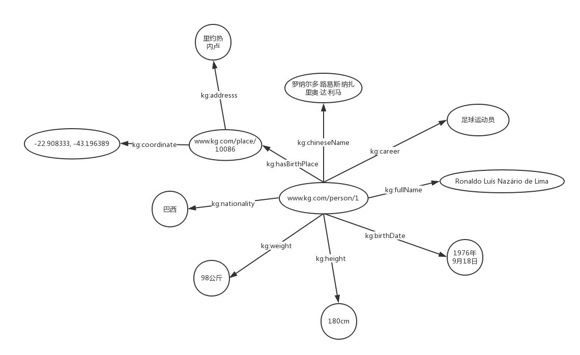
match p = (n) -[*1..2] -> (m) where n.name='特朗普' return p
match p =  ({name: '特朗普'}) - [*1..2] -> () return p # 简化
match p = (n)-[m]->(q) where m.name = '丈夫' return n,q skip 10 limit 5
match p = (n)-[:丈夫]->(q) return n,q skip 10 limit 5 # 简化
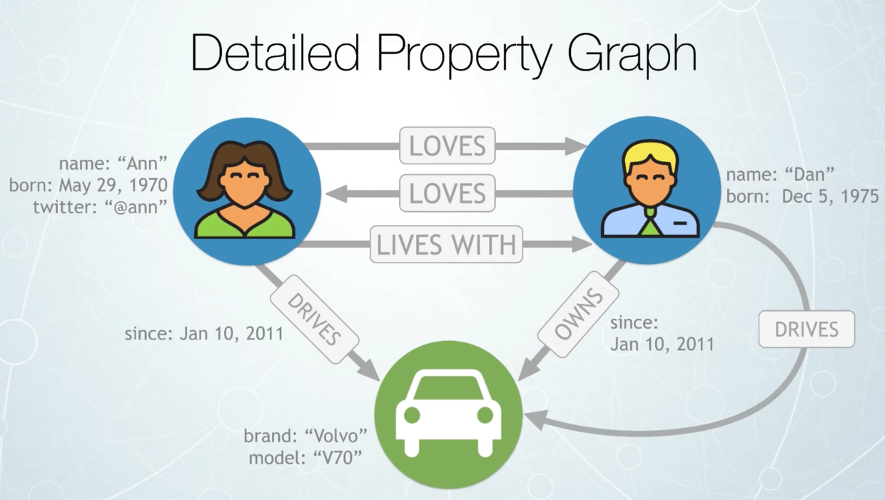
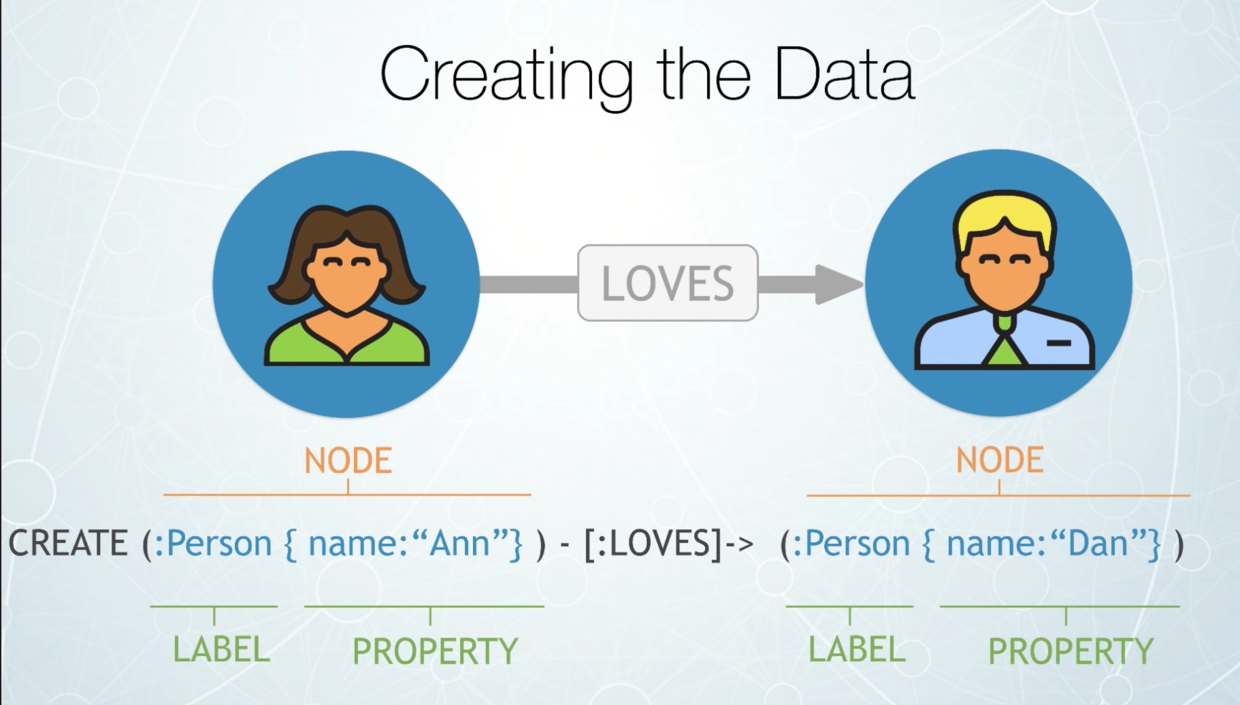
解读:

  1. 上面写法很简略,注意观察一下
  2. 又一次演示了直接用json来做where和单独用where关键字的写法区别(要多命名一个变量)
  3. p跟n的区别,p是返了整个网络,如果return n,那么就是n自身(一个节点)。

4, 但是如果return n, m,那么又把一层网络给select出来了 5. [*1..2]表示跟踪两层 6. 如果不需要对n,m进行where,set操作,可以不设置变量 7. relationship也可以过滤,也有name等属性 8. limit, skip 等用法

Tabular Results

MATCH (p:Person {name: "Tom Hanks"}) - [r:ACTED_IN|DIRECTED] -> (m:Movie)
RETURN p,r,m
RETURN p.name, type(r), m.title

前者返回Graph,后者返回表格数据

Update

P.S. where是对属性做限制,所以查询条件既可以写在属性里,也可以用where语句来做过滤.

要对查询结果进行修改,用set(有则改,无则加)

MATCH
(:Person {name: "张三"}) - [:LOVES] -> (p:Person)
RETURN
p

MATCH
(p1:Person) - [:LOVES] -> (p2:Person)
WHERE
p1.name = "张三"
SET
p2.age = 33  # set by property
# or
p2 += {age: 33, height: 180}  # set by JSON
RETURN
p2

可以把Neo4j理解为命名实体识别(NER),即你创造一句话,为句子里的每个实体打上标签,然后你想要谁就用实体标签把它取出来。

比如“张三爱李四”:

step1: 写框架
CREATE () - [] -> ()
step2: 填节点和关联
CREATE (:Person {name: "张三"}) - [:LOVES] -> (:Person {name: "李四"})

而你要问张三爱谁:

MATCH
(:Person {name: "张三"}) - [:LOVES] -> (p:Person)
RETURN
p

看到查询语句了吗?除了CREATE, MATCH等关键词,句子顺序是完全一样的,也就是说,一直是在“陈述”一件事。

而事实上,这个NER在知识图谱中表示为RDF

Delete

match p=(n) where n.name = '小明' detach delete n

Query

最短距离

MATCH
  (martin:Person {name: 'Martin Sheen'}),
  (oliver:Person {name: 'Oliver Stone'}),
  p = shortestPath((martin)-[*..15]-(oliver)) # 1
  p = allShortestPath(....) # 2
  WHERE none(r IN relationships(p) WHERE type(r) = 'FATHER') # 3
RETURN p
  1. 限定了15层
  2. Finds all the shortest paths between two nodes.
  3. 排除了关系typeFATHER

给你们看一下一个relationships长啥样:

{
  "identity": 36629,
  "start": 31343,
  "end": 33922,
  "type": "author->title",
  "properties": {
"name": "author->title"
  }
}

模糊匹配(%)

match p = (a)-[*1..2]->(b:content) where a.name = '李白' and b.name =~ '.*明月.*' return a,b

.*就相当于sql里的%

get by id

MATCH (n)
WHERE id(n) IN [0, 3, 5]
RETURN n
  1. id(n) -> search with id
  2. multiple id use in

outer join (optional relationships)

match (a:author {name:'李白'})
optional match (a)-->(b)
return b

在实例中,b包含了两种实例:

  1. title
  2. introduce

等同于sql中user表outer join了两个表(title, introduce)

HMM、NER、PoS、Viterbi笔记

开局一句话,隐马尔可夫,就是在“溯源”,即产生你这个现象的源头在哪。

  • 比如你掷出的这个显示为6的骰子,是来自于六面体的还是四面体的,或是来自于普通的还是灌铅了的
  • 又比如你一句话里的某一个词,它是处于开始位置还是中间位置,或是它是一个人名还是一个地点或是一个介词

任何一种表现形式,都有一个它的“原因”或“属性”。 现在正式开始,来自我能理解的网络资料,我的课程,以及一些思考

首先几个基础概念:

命名实体识别(NER)

实体:人物(PER),地点(LOC),等 BIOES: 开始(Begin), 中间(Inner), 结尾(E),单个(Single),其它(Other)

比如人名:张北京,就可以被识别为$\Rightarrow$ B-PER, I-PER, E-PER

Part-of-Speech Tagging(词性标注)

词性标注是为输入文本中的每个词性标注词分配词性标记的过程。标记算法的输入是一系列(标记化的)单词和标记集,输出是一系列标记,每个标记一个。

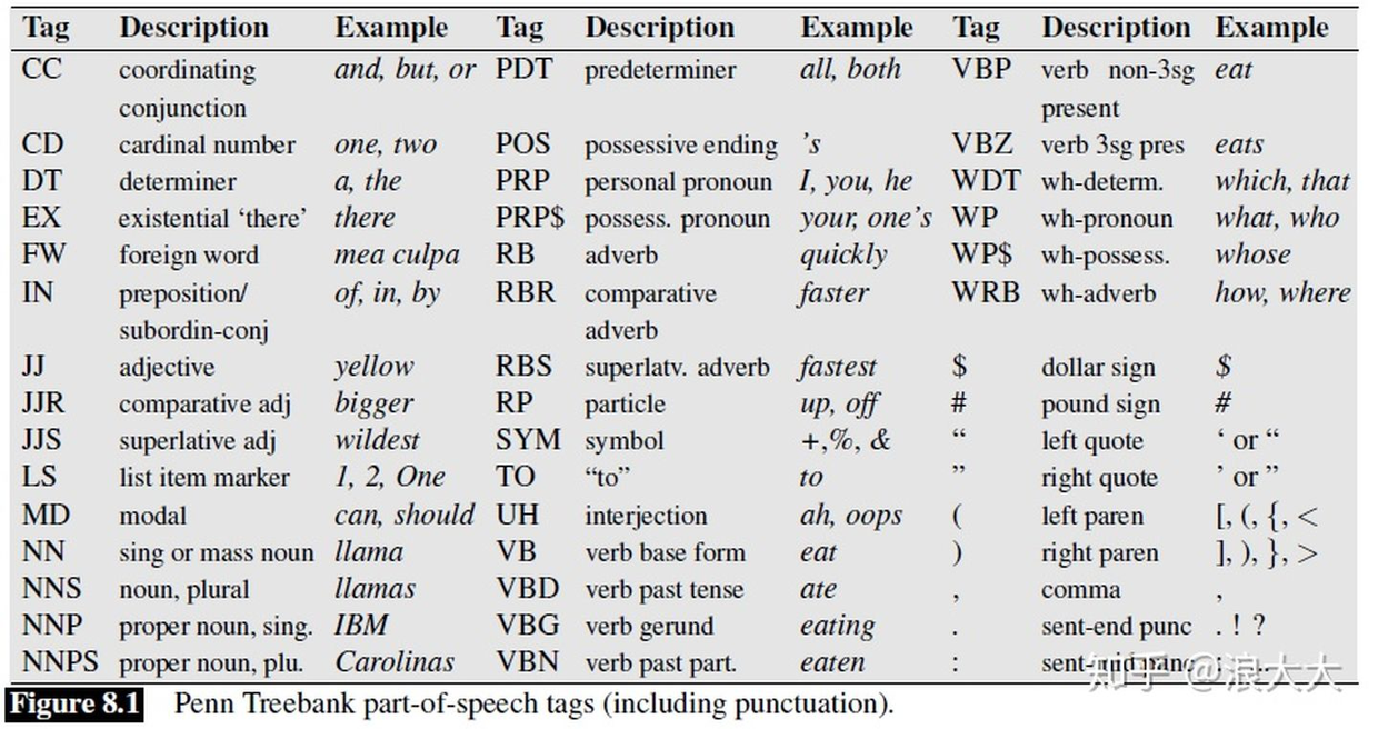
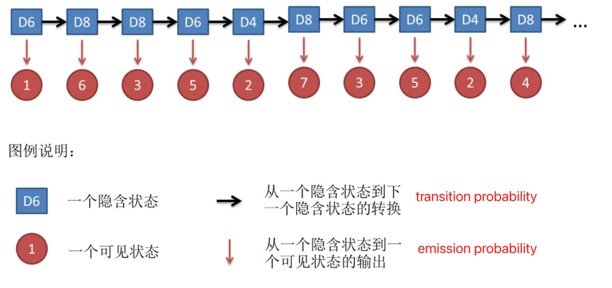
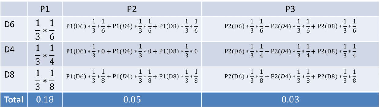
标记是一项消除歧义的任务;单词是模糊的,有不止一个可能的词性(歧义),我们的目标是为这种情况找到正确的标签。例如,book可以是动词(book that flight),也可以是名词(hand me that book)。That可以是一个限定词(Does that flight serve dinner),也可以是一个补语连词(I thought that your flight was earlier)。后置标记的目标是解决这些分辨率模糊,为上下文选择合适的标记
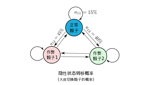
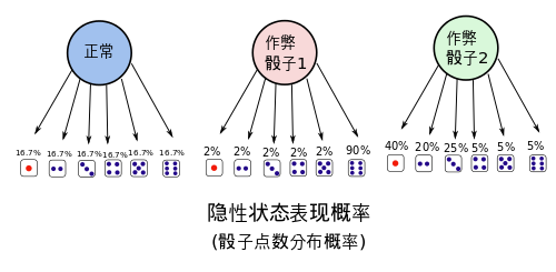
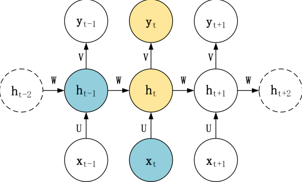
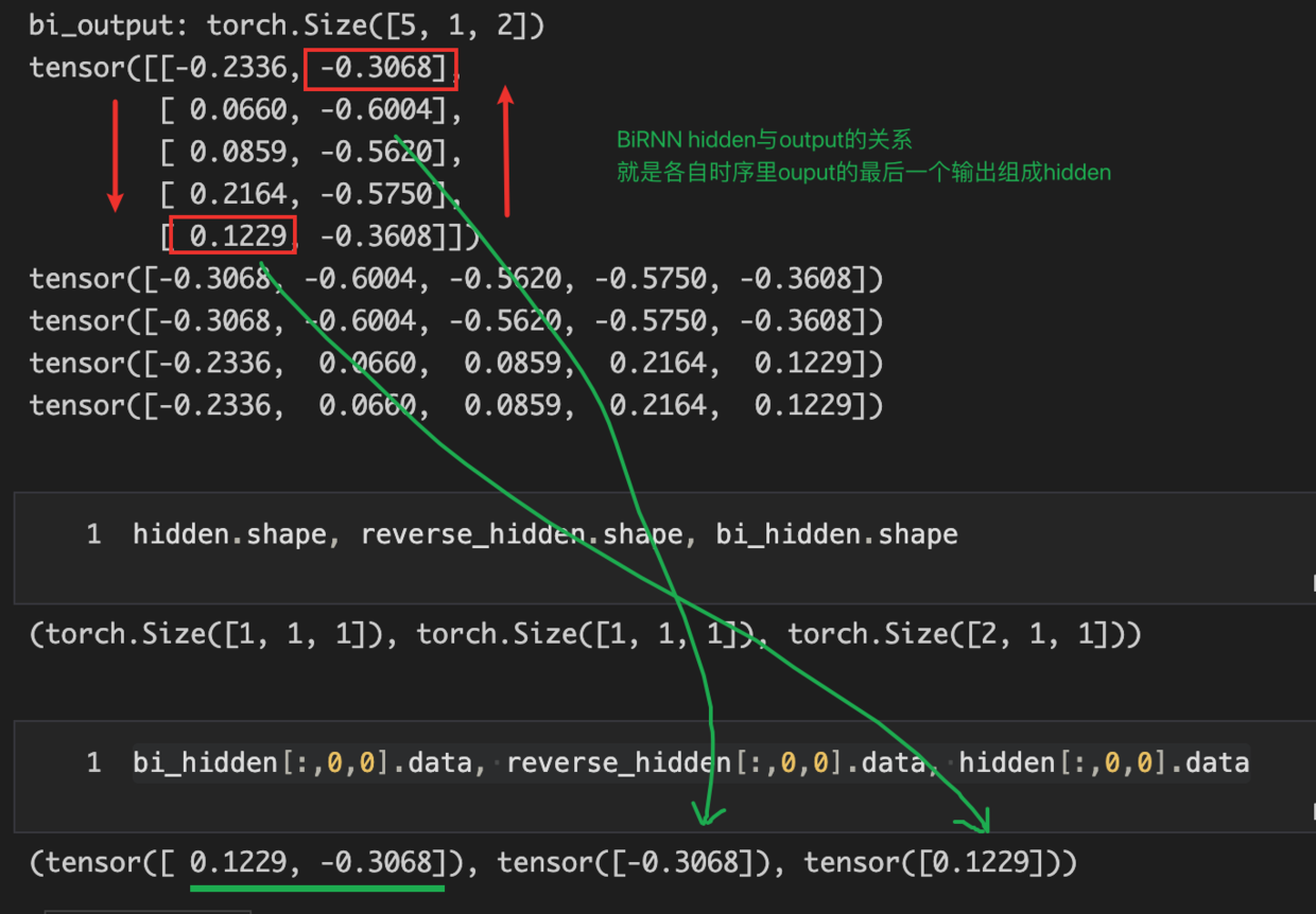
Sequence model

Sequence models are central to NLP: they are models where there is some sort of dependence through time between your inputs.

  • The classical example of a sequence model is the Hidden Markov Model for part-of-speech tagging. (词性标注)
  • Another example is the conditional random field.

HMM模型的典型应用是词性标注

词性标注语料库是统计标注算法的关键训练(和测试)集。三个主要的标注语料库始终用于训练和测试英语词性标注器。

  1. 布朗语料库是1961年在美国出版的500篇不同体裁的书面文本的100万单词样本。
  2. 《华尔街日报》语料库收录了1989年发表在《华尔街日报》上的100万个单词。
  3. 总机语料库由1990-1991年收集的200万字电话对话组成。语料库的创建是通过在文本上运行一个自动的词性标记,然后由人工注释器手工更正每个标记。

HMM

HMM是一个序列模型(sequence model)。序列模型或序列分类器是一个模型,其工作是为序列中的每个单元分配一个标签或类,从而将一个观察序列(观察状态)映射到一个标签序列(隐藏状态)。HMM是一种概率序列模型:给定一个单位序列(单词、字母、语素、句子等等),它计算可能的标签序列的概率分布,并选择最佳标签序列。

  • 3个骰子,6面体,4面体,8面体(D6, D4, D8)
  • 每次随机选出一个骰子投掷,得到一个数字
  • 共十次,得到10个数字
  1. 可见状态链:10次投掷得到10个数字(1,3,5...)$\Rightarrow$对应你看得的10个单词
  2. 隐含状态链:每一次投掷都有可能拿到三种骰子之一,(D6, D6, D4...) $\Rightarrow$对应为每个单词的词性
  3. 转换概率(transition probability):隐含状态之间的概率($\Rightarrow$对应为语法):
    • 每一次拿到某种骰子之后,下一次拿到三种骰子的概率([1/3,1/3,1/3],...)
    • 或者说主动决策下一次用哪个骰子的概率[a,b,c...] (相加为1)
  4. 可见状态之间没有转换概率
  5. 输出概率(emission probability):隐含状态和可见状态之间的概率,比如D4下1的概率为1/4,D6下为1/6 (表现概率,激发概率,多种翻译)

应用HMM模型时候,往往是缺失了一部分信息的,

  • 有时候你知道骰子有几种,每种骰子是什么,但是不知道掷出来的骰子序列;
  • 有时候你只是看到了很多次掷骰子的结果,剩下的什么都不知道。

如何应用算法去估计这些缺失的信息,就成了一个很重要的问题,这也是HMM模型能做的几件事:

Decoding

解码的过程就是在给出一串序列和已知HMM模型的情况下,找到最可能的隐性状态序列。

比如结果是:1 6 3 5 2 7 3 5 2 4, 求最可能的骰子序列

Viterbi algorithm

  1. 掷出1的最大概率是4面体: P1(D4) = P(1|D4) * P(D4) = 1/4 * 1/3
  2. 掷出6的最大概率是 P2(D6) = P(6|D6) * P(D6) = 1/6 * 1/3
  3. 连续1,6的概率就成了1的概率 * 2的概率 P2(D6) = P1(D4) * P2(D6) = 1/216
  4. 1,6,3 => P3(D4) = P2(D6) * P(3|D4) * P(D4) = $\frac{1}{216} \cdot \frac{1}{3} \cdot \frac{1}{4}$
  5. and so on
  6. 但这个例子忽略了转移概率,即P(D6|D4), P(D4|D6,D4),或者说默认了转移概率就是1/3,即每次挑中三个骰子的机率均等。

Evaluation

根据条件和序列结果求这一序列的概率是多少,比如三种骰子,投出了1,6,3的结果:

  • 第1列表示第一次投掷得到1的可能性和为0.18
  • 第2列为1 6的的可能性和为0.05
  • 第3列为1 6 3的可能性和为0.03

如果远低于或远高于这个概率,必然有做过手脚的骰子。

转移概率的矩阵表示

这次假定不同的骰子是用来作弊的,作弊者会根据情况来挑选骰子,这样转移概率就不可能是均等的了:

很幸运,这么复杂的概率转移图,竟然能用矩阵表达:

$$A = \begin{bmatrix} 0.15 & 0.45 & 0.4 \\ 0.25 & 0.35 & 0.4 \\ 0.10 & 0.55 & 0.35 \end{bmatrix} $$

既然是3行3列,显然$A_{ij}$就是从i切换到j的概率,比如$A_{12}$ 就应该是这个人把骰子从作弊骰子1切换到2的概率。

相应地,发射概率(即不同骰子摇出的点数的概率)也能表示为矩阵:

$$B = \begin{bmatrix} 0.16 & 0.16 & 0.16 & 0.16 & 0.16 & 0.16 \\ 0.02 & 0.02 & 0.02 & 0.02 & 0.02 & 0.90 \\ 0.40 & 0.20 & 0.25 & 0.05 & 0.05 & 0.05 \\ \end{bmatrix} $$

现在有了转移概率和发射概率,我们再来看看前面的掷出1,6,3的骰子的概率: 骰子设为D1 D2 D3, 每一轮的可能性为P1 P2 P3, 则P = P3D1 + P3D2 + P3D3 即第3轮时3种骰子能投出3的概率和

我来推导一下P3D1怎么来的,上面的表格是我从别人的博客里复制的,这里就不做一个一模一样的图了,我们一步步来吧:

  • 第一次投掷每个骰子的概率应该是隐含了各为1/3吧?(这个好像叫"初始隐状态" $\pi$)
  • P1D1 = 0.16 * 0.33, 即1/3概率拿到D1,0.16概率投出1,同理:
    • P1D2 = 0.02 * 0.33
    • P1D3 = 0.40 * 0.33
  • P2D1 =
    • P1D1 * $A_{00}$ * $B_{05}$ = P1D1 * 0.15 * 0.16 即P1D1前提下,乘上D1换到D1的概率,再乘上D1选出6的概率
    • $+$
    • P1D2 * $A_{10}$ * $B_{05}$ = P1D1 * 0.25 * 0.16 即P1D2前提下,乘上D2换到D1的概率,再乘上D1选出6的概率
    • $+$
    • P1D3 * $A_{20}$ * $B_{05}$ = P1D1 * 0.10 * 0.16 即P1D3前提下,乘上D3换到D1的概率,再乘上D1选出6的概率
    • 以此类推得到P2D2, P2D3
  • P3D2 = (D1的概率太平均,这次换个D2来演示
    • P2D1 * $A_{01}$ * $B_{12}$ = P2D1 * 0.45 * 0.02 即P2D1前提下,乘上D1换到D2的概率,再乘上D2选出3的概率
    • $+$
    • P2D2 * $A_{11}$ * $B_{12}$ = P2D1 * 0.35 * 0.02 即P2D2前提下,乘上D2换到D2的概率,再乘上D2选出3的概率
    • $+$
    • P2D3 * $A_{21}$ * $B_{12}$ = P2D1 * 0.35 * 0.02 即P2D3前提下,乘上D3换到D2的概率,再乘上D2选出3的概率
    • 以此类推得到P3D1, P3D2
  • P = P3D1 + P3D2 + P3D3

$$ \sum_{r\in R}\prod_t^TP(v(t)|w_r(t)) | w_r(t-1)) $$

  • v: visible 可见序列
  • w: 隐性状态序列
  • R: 所有隐状态的可能性
  1. t-1隐状态前提下得到t的概率(转移概率)如D2换到D3的概率
  2. 上一概率前提下得到v(t)的概率,如D3扔出1的概率
  3. 一种隐状态下出序列的结果为累乘
  4. 所有隐状态下出该序列的结果为3的累加

简单来说:

  1. 可见序列$v(t)$的概率依赖当前$t$下的隐状态(比如是不是作弊了的骰子)$w_r(t)$
    • 得到:$P(v(t)\ \color{red}|\ w_r(t))$
  2. 当前隐状态$w_r(t)$又有两个特征:
    1. 由$w_r(t-1)$转换而来的: $P(v(t)|w_r(t))\color{red}{|}w_r(t-1)$
    2. $T$是链式的,概率累乘: $\color{red}{\prod_t^T}P(v(t)|w_r(t)) | w_r(t-1))$
  3. 最后一步时的隐状态显然是几种之一,累加起来就是所有可能性:
    • $\color{red}{\sum_{r\in R}}\prod_t^TP(v(t)|w_r(t)) | w_r(t-1))$

应用

  1. 初始概率

BMES为例(参考NER),把其认为是隐状态,然后认为每个词(里的字)是由隐状态产生的。

B对应的字可能有“”,“”,等等,能作为词语打头的字都可能由隐状态B产生,其它状态依次类推。

就像我们三种骰子的初始概率,完全取决于每种骰子占总数的多少一样,HHM应用到语言模型里,初始概率就是先把文字全部用BMES表示,然后分别数出个数,与总数做个对比。(此时已经可以判断出ME的概率只能是0了。

  1. 转移概率

应该是4个循环吧,每次把当前状态后面跟上四个状态的情况都数出来,就是一个隐状态到其它四个状态的转移概率,四行拼到一起就是一个转移概率的矩阵,类似上面的三种骰子互相切换的矩阵。

也可以用字典,比如 BE BS BB BM等共16个键,两两遍历整个字符串完后,16个count就出来了,group后就能得到概率了。

  1. 观测概率(发射概率)

这个就是每一个隐状态下对应不同表面文字的概率了,比如:{s:{"周": 0.3357, "爬":0.00003}...}

要知道,三种概率里面是有很多0的,意思就是在现有的语法体系里面不可能出现的场景,比如第一个字不可能是M和E,B后面不可能跟S,B,而M后面不可能跟B,S,以及S后面不可能跟M,E等,再比如假如哪个字永远不可能是第一个字,那么它的观测概率在S里面就永远是0,等等。

这里要计算的话,因为隐状态是用文字推断出来的,所以这个映射关系还在,那么整理一下两个数组就能把每个隐状态能对应的文字全部映射上了。


以下是我课程里的笔记,理解了上面的内容,理解下面是没有任何障碍的。

viterbi in NLP

$\overbrace{ 0 \xrightarrow[农]{2.5} 1 \xrightarrow[产]{4.0} 2 }^{1.4} \xrightarrow[物]{2.3} 3$

$0 \xrightarrow[农]{2.5} \underbrace{ 1 \xrightarrow[产]{4.0} 2 \xrightarrow[物]{2.3} 3 }_{2.1}$

数字画圈的写法 $\enclose{circle}{3}$ 这个生成器暂不支持

  • node: $\enclose{circle}{2}$ ,圆圈,就是位置索引
  • edge: 词, 箭头,很好理解:string[0,1] = '农'
  • Each edge weight is a negative log probality
    • -log(P(农)) = 2.5
    • -log(P(产)) = 4.0
    • -log(P(农产)) = 1.4
    • -log(P(产物)) = 2.1
  • Each path is a segmentation for the sentence
  • Each path weight is a sentence unigram negative log probability
    • -log(P(农产)) + -log(P(物)) = 1.4 + 2.3 = 3.7
    • 农 + 产 + 物 = 2.5 + 4.0 + 2.3 = 8.8
    • 农 + 产物 = 2.5 + 2.1 = 4.6

two step

1.前向,从左往右,找到最佳路径的分数 2.后向,从右往左,创建一条最佳路径

forward algorithm

pseudo code

best_score[0]=0
for each node in the graph (ascending order)
  best_score[node] = 
  for each incoming edge of node
    score=best_score[edgeprev_node]+edge.score
    if score < best_score[node]
      best_score[node]=score
      best_edge[node] =edge

example:

  • 初始节点打分0,其它节点打分为$\infty$
  • 每个节点打分由其(incoming edge)(即来源箭头)和来源节点的打分构成
  • 如果有多个来源,则计算出该来源的得分,与该节点当前的得分做对比,取得分低的那个
  • 把该节点的分值和来源edge存到该节点上(edge就是词)。
  1. 简单来说,还是和之前的骰子一样,每一次算出到当前节点的最低分数的路径。
  2. 上图中,我们就把e1, e2, e5选出来了,这个过程中,删除了e3, e4这几条路径
  3. best_score=(0.0, 2.5, 1.4, 3.7), best_edge = (NULL, e1, e2, e5)
  4. 用字典来把Node映射上去:{0:(0.0, NULL), 1:(2.5, e1), 2:(1.4, e2), 3:(3.7, e5)}

backward algorithm

best_path=[]
next_edge=best_edge[best_edge.length-1]
while next_edge != NULL
  add next_edge to best_path
  next_edge =best_edge[next_edge.prev_node]
reverse best path

举例:

  • 从图片可知,path就是edge
  • 初始path是空,[]
  • forward的结果字典里找到node 3的best_edge,就是e5 [e5]
  • e5的来源的是node 2
  • 从字典里找到2的best_edge,是e2 [e5, e2]
  • e2的来源是node 0
  • 0的best_edge是NULL,结束递归
  • reverse: [e2, e5]

这个很好理解

  1. 0到农,到农产,到农产物的概率,表示为0.0+ -log(p(农/农产/农产物))
  2. 在农的前提下,就有农到产,和农到产物:best(1) + -log(P(产/产物))
  3. 在产的前提下,就只有best(2) + -log(P(物))了

应用到NLP:

这里就是把node, egde具体了一下:

  1. 多包了一层for-each,意思是前面的代码是处理一行的
  2. node对应是单词结尾(word_end),其实就是一个index,前面说过了
  3. edge对应是单词(word),前面也说过了,即string[5,7]的意思
  4. score由uni-gram来计算
  5. 计算上,就是找到以基准字当作单词结尾,然后前面的字跟它拼起来的所有可能性,找最低分:
    • 比如abcdefg, 如果当前是e,那么分别比较:abced, bcde, cde, de
  6. 接上例,输出结果应该这么解读:
    • 以b为结尾的单词,最有可能的是xxx, 它的得分是,它的索引是,
    • 以c为结尾的单词,最有可能是bc或是abc,它的得分是,bc/abc的索引是(1,2),这样
  1. 显然这里已经知道edge不知道是一个词,而且是一个词的首尾边界
  2. 也知道存到best_edges里面的其实就是词的位置索引
  3. 反向的时候,从最后一个索引找到得分最低的词,再从这个单词向前找,一直找到
    • 所以next_edge[0]其实就是当前单词词首,[1]就是词尾
    • 所以把当前单词存进去后,向前搜索就要以next_edge[0]为字典,找对应的best_edge
    • 再从best_edge里面解析出最合适的单词的首尾索引,存到结果数组里

Mac远程Windows-10里用Anaconda装的Jupyter-lab

家里台式机配置比笔记本好多了,但又习惯了苹果本,怎么在小本本上直接跑windows上的jupyter呢?

首先,给Windows 10 装上OpenSSH

如果你不是用的Anaconda等虚拟环境而是把python和jupyter lab装在了本机以及写在了path里,理论上你用ssh连上windows后在shell里直接jupyter lab就好了,可是我是用了Anaconda的,ssh进去以及windows自身的命令行环境里都是执行不了conda和jupyter的

可能仅仅只是path的原因,但应该没这么简单,考虑到端口转发已经能实现我的目的了,就不深究了。

这时使用ssh的本地端口转发功能可以达到目的:

$ ssh -L 2121:host2:21 host3

即把host3的端口21转发到host2的2121上去,当然,大多数情况下host2就是本机,那么localhost就好了:

$ ssh -L 8000:localhost:8889 windows-server

当然,8889是你在windows上运行--no-browser的jupyter lab设定的端口:

jupyter lab --no-browser --post=8889

Semi supervised Learning

李宏毅机器学习2021spring的家庭作业里面有一个Semi-supervised Learning的任务。

具体来说,就是一个图片分类的任务(11个食品类别),但只给了你几百个有标注的图片,同时,还给了你几千张没有标的图片(用来训练,而不是测试)。

思路也很简单,既然样本量过小,我们就得自己扩充样本量,但这次不是用数据增广(Augumentation),而是自己造样本:

  1. 用小样本训练一个模型,用这个模型来predict没有标注的图片(文本有补述)
  2. 对预测输出的11个类别softmax后,观察最大值,如果大于你设定的某个threshold,比如0.68,就把该图片和最大值所映射的类别当成一组真值添加到训练集里去
  3. 我用的是torch.utils.data里的TensorDataset来构建手动创建的增强数据集,然后用了ConcatDataset与原训练集拼接:
from torch.utils.data import TensorDataset

def get_pseudo_labels(dataset, model, threshold=0.65):
    # This functions generates pseudo-labels of a dataset using given model.
    # It returns an instance of DatasetFolder containing images whose prediction confidences exceed a given threshold.
    # You are NOT allowed to use any models trained on external data for pseudo-labeling.
    device = "cuda" if torch.cuda.is_available() else "cpu"

    # Construct a data loader.
    data_loader = DataLoader(dataset, batch_size=batch_size, shuffle=False)

    # Make sure the model is in eval mode.
    model.eval()
    # Define softmax function.
    softmax = nn.Softmax(dim=-1)

    # Iterate over the dataset by batches.
    images = torch.Tensor([])
    targets = torch.Tensor([])
    for batch in tqdm(data_loader):
        img, _ = batch

        # Forward the data
        # Using torch.no_grad() accelerates the forward process.
        with torch.no_grad():
            logits = model(img.to(device))

        # Obtain the probability distributions by applying softmax on logits.
        probs = softmax(logits)

        # ---------- TODO ----------
        # 在这里根据阈值判断是否保留
        # Filter the data and construct a new dataset.
        for idx, prob in enumerate(probs):
            c = torch.argmax(prob)
            if prob[c] > threshold:
                torch.cat((images, img[idx]))   # 用索引选出对应的图片
                torch.cat((targets, torch.tensor(c))) # 用最大值索引当class

    dataset = TensorDataset(images, targets)  # 拼成tensor dataset

    # # Turn off the eval mode.
    model.train()
    return dataset

使用:

pseudo_set = get_pseudo_labels(unlabeled_set, model)

# Construct a new dataset and a data loader for training.
# This is used in semi-supervised learning only.
concat_dataset = ConcatDataset([train_set, pseudo_set]) # 拼接两个dataset(只要有感兴趣的两组数组即可)
train_loader = DataLoader(concat_dataset, batch_size=batch_size, shuffle=True, num_workers=4, pin_memory=True)

看来,所谓的半监督仍然是有监督,对于没有标注的数据,仍然要想办法用已有数据去为它打标,接下来就是普通的监督学习了。


最后,在实际的demo代码中,能看到并不是我最初理解的“先用小样本训练好一个模型”,再用它来过滤un-labeled样本,增广到训练集去,即对训练集的增广是一劳永逸的(像别的增广方案一样)

而是每一个epoch里面都重新去增广一次,这个思路更类似于GAN(生成对抗网络),generatordiscriminator是一起训练的。

也所以,第一次去增广的时候,其实就是一个初始化的model,也就是说,一个比较垃圾的数据集(当然,初始化的model未必能预测出置信度高的结果,以至于并不会有太多pseudo labels进入训练集)

因此,相比较纯监督学习,假如训练集是2000条,那么整个epoch轮次里,都是2000条数据在训练;而半监督学习里,可能是200, 220, 350, 580, 1000, 1500...这样累增的样本量(随着模型越来越好,置信度应该是越来越高的),如果epoch数量不够,可能并没有在相同2000左右的样本量下得到足够的训练

RNN梯度消失与梯度爆炸推导

$$ \large \begin{aligned} h_t &=\sigma(z_t) = \sigma(Ux_t+Wh_{t-1} + b) \ y_t &= \sigma(Vh_t + c) \end{aligned} $$

梯度消失与爆炸

假设一个只有 3 个输入数据的序列,此时我们的隐藏层 h1、h2、h3 和输出 y1、y2、y3 的计算公式:

$$ \large \begin{aligned} h_1 &= \sigma(Ux_1 + Wh_0 + b) \\ h_2 &= \sigma(Ux_2 + Wh_1 + b) \\ h_3 &= \sigma(Ux_3 + Wh_2 + b) \\ y_1 &= \sigma(Vh_1 + c) \\ y_2 &= \sigma(Vh_2 + c) \\ y_3 &= \sigma(Vh_3 + c) \end{aligned} $$

RNN 在时刻 t 的损失函数为 Lt,总的损失函数为 $L = L1 + L2 + L3 \Longrightarrow \sum_{t=1}^TL_T$

t = 3 时刻的损失函数 L3 对于网络参数 U、W、V 的梯度如下:

$$ \begin{aligned} \frac{\partial L_3}{\partial V} &= \frac{\partial L_3}{\partial y_3} \frac{\partial y_3}{\partial V} \\ \frac{\partial L_3}{\partial U} &= \frac{\partial L_3}{\partial y_3} \frac{\partial y_3}{\partial h_3} \frac{\partial h_3}{\partial U} + \frac{\partial L_3}{\partial y_3} \frac{\partial y_3}{\partial h_3} \frac{\partial h_3}{\partial h_2} \frac{\partial h_2}{\partial U} + \frac{\partial L_3}{\partial y_3} \frac{\partial y_3}{\partial h_3} \frac{\partial h_3}{\partial h_2} \frac{\partial h_2}{\partial h_1} \frac{\partial h_1}{\partial U} \\ \frac{\partial L_3}{\partial W} &= \frac{\partial L_3}{\partial y_3} \frac{\partial y_3}{\partial h_3} \frac{\partial h_3}{\partial W} + \frac{\partial L_3}{\partial y_3} \frac{\partial y_3}{\partial h_3} \frac{\partial h_3}{\partial h_2} \frac{\partial h_2}{\partial W} + \frac{\partial L_3}{\partial y_3} \frac{\partial y_3}{\partial h_3} \frac{\partial h_3}{\partial h_2} \frac{\partial h_2}{\partial h_1} \frac{\partial h_1}{\partial W} \\ \end{aligned} $$

其实主要就是因为:

  • 对V求偏导时,$h_3$是常数
  • 对U求偏导时:
    • $h_3$里有U,所以要继续对h3应用chain rule
    • $h_3$里的$W, b$是常数,但是$h_2$里又有U,继续chain rule
    • 以此类推,直到$h_0$
  • 对W求偏导时一样

所以:

  1. 参数矩阵 V (对应输出 $y_t$) 的梯度很显然并没有长期依赖
  2. U和V显然就是连乘($\prod$)后累加($\sum$)

$$ \begin{aligned} \frac{\partial L_t}{\partial U} = \sum_{k=0}^{t} \frac{\partial L_t}{\partial y_t} \frac{\partial y_t}{\partial h_t} (\prod_{j=k+1}^{t}\frac{\partial h_j}{\partial h_{j-1}}) \frac{\partial h_k}{\partial U} \\ \frac{\partial L_t}{\partial W} = \sum_{k=0}^{t} \frac{\partial L_t}{\partial y_t} \frac{\partial y_t}{\partial h_t} (\prod_{j=k+1}^{t}\frac{\partial h_j}{\partial h_{j-1}}) \frac{\partial h_k}{\partial W} \end{aligned} $$

其中的连乘项就是导致 RNN 出现梯度消失与梯度爆炸的罪魁祸首,连乘项可以如下变换:

  • $h_j = tanh(Ux_j + Wh_{j-1} + b)$
  • $\prod_{j=k+1}^{t}\frac{\partial h_j}{\partial h_{j-1}} =\prod_{j=k+1}^{t} tanh' \times W$

tanh' 表示 tanh 的导数,可以看到 RNN 求梯度的时候,实际上用到了 (tanh' × W) 的连乘。当 (tanh' × W) > 1 时,多次连乘容易导致梯度爆炸;当 (tanh' × W) < 1 时,多次连乘容易导致梯度消失。

RNN中bidirectional和num_layer对output和hidden形状的影响

Batch first

首先,我们要习惯接受batch_first=False(就是默认值)的思维,因为NLP中批量处理句子,是每一句取第一个词,第二个词,以此类推。 按我们习惯的把数据放在同一批(即batch_first=True)的思路虽然可以做到(善用切片即可),但是绕了弯路。但是如果第1批都是第1个字,第2批全是第2个字,这会自然很多(行优先)。

所以至少Pytorch内部,你设了True,内部也是按False来处理的,只是给了你一个语法糖(当然你组织数据就必须按True来组织了。

看个实例:

  1. 假定批次是64,句长截为70,在还没有向量化的数据中,那么显然一次的输入应该为(70x64),批次在第2位
  2. 注意第一行,全是2,这是设定的<bos>,这已经很好地表示了在行优先的系统里(比如Matlab就是列优先),会自然而且把每句话的第一个词读出来的设定了。
# 我用的torchtext的Field进行演示, SRC是一个Field
[SRC.vocab.itos[i] for i in range(1,4)]  
['<pad>', '<bos>', '<eos>']
  1. 可见,2是开始,3是结束,1是空格(当然这是我设置的)
  2. 同时也能注意到,最后一行有的是3,有的是1,有的都不是,就说明句子是以70为长度进行截断的,自然结束的是3,补<pad>的是1,截断的那么那个字是多少就是多少
  3. 竖向取一条就是一整句话,打印出来就是箭头指向的那一大坨(共70个数字)
  4. 对它进行index_to_string(itos),则还原出了这句话
  5. nn.Embedding做了两件事:
  • 根据vocabulary进行one-hot(稀疏)$\rightarrow$ 所以你要告诉它词典大小
  • 然后再embedding成指定的低维向量(稠密)
  • 所以70个数字就成了70x300,拼上维度,就是70x64x300

既然讲到这了,多讲两行,假定hidden_dim=256, 一个nn.RNN会输出的outputshidden的形状如下:

>>> outputs.shape
torch.Size([70, 64, 256])
>>> hidden.shape
torch.Size([1, 64, 256])
  1. 即300维进去,256维出来,但是因为句子有70的长度,那就是70个output,hidden是从前传到后的,当然是最后一个
  2. 也因此,如果你不需要叠加多层RNN,你只需要最后一个字的output就行了outputs[-1,:,:], 这个结果送到全连接层里去进行分类。

自己写一个RNN

其实就是要自己把上述形状变化做对就行了。就是几个线性变换,所以我们用nn.Linear来拼接:

  1. input: 2x5x3 $\Rightarrow$ 5个序列,每一个2个词,每个词用3维向量表示
  2. hidden=10, 无embedding,num_class=7
  3. 期待形状:
  • output: 2x5x7
  • hidden:1x5x10
class RNN(nn.Module):
    def __init__(self, input_size, hidden_size, output_size):
        super(RNN, self).__init__()
        self.hidden_size = hidden_size
        self.i2h = nn.Linear(input_size + hidden_size, hidden_size)
        self.i2o = nn.Linear(input_size + hidden_size, output_size)
        self.softmax = nn.LogSoftmax(dim=1)

    def forward(self, input, hidden):
        combined = torch.cat((input, hidden), 2)
        # input shape: (2, 5, 3)
        # hidden shape: (2, 5, 10)
        # combine shape (2, 5, 13)
        hidden = self.i2h(combined)
        output = self.i2o(combined)
        output = self.softmax(output)
        return output, hidden

    def initHidden(self):
        return torch.zeros(1, self.hidden_size)

hidden_size = 10
num_class = 7
input = torch.randint(0,10,(2,5,3))

rnn = RNN(input.size(2),hidden_size,num_class)
out, hid = rnn(input, torch.zeros(2, 5, hidden_size))
out.shape, hid.shape

output:

(torch.Size([2, 5, 7]), torch.Size([2, 5, 10]))

可见,output是一样的,hidden的形状不一样,事实上每一个字确实是会产生hidden的,但是pytorch并没有把它返出来(消费掉就没用了)。这里就pass了,我们主要是看一下双向和多层的情况下形状的变化,下面我们用pytorch自己的RNN来测试。

num_layers

import torch
import torch.nn as nn
torch.manual_seed(3)
num_layers = 3
batch_size = 2
rnn = nn.RNN(input_size=3, hidden_size=12, num_layers=num_layers, batch_first=False)
h0 = torch.randn(num_layers, batch_size, 12) # 几层就需要初始几个hidden
x0 = torch.rand(5, batch_size, 3) # input: 5x3 -> 1x12 # N个批次, 5个序列(比如5个字,每个字由3个数字的向量组成)
o, h = rnn(x0, h0) # 5个output, 一个final hidden
print('output shape', o.shape)
print('hidden shape', h.shape)

输出:

output shape torch.Size([5, 2, 12])  # 2个批次,5个词,12维度输出
hidden shape torch.Size([3, 2, 12]) # 3层会输出3个hidden,2个批次

加上embedding, RNN改成GRU

# 这次加embedding
# 顺便把 RNN 改 GRU
vocab_size = 5
embed_size = 10
hidden_size = 8
batch_size = 3
# 要求词典长度不超过5,输出向量长度为10
emb = nn.Embedding(vocab_size, embed_size) 
# 输入为embeding维度,输出(和隐层)为8维度
rnn = nn.GRU(embed_size, hidden_size, batch_first=False, num_layers=2)
# 这次设了num_layers=2,就要求有两个hidden了
h0 = torch.rand(2, batch_size, hidden_size)
# 因为数据会用embedding包一次,所以input没有了维度要求(只有大小要求,每个数字要小于字典长度)
x0 = torch.randint(1, vocab_size, (5, batch_size)) 
e = emb(x0)
print('input.shape:', x0.shape)
print('embedding.shape:', e.shape)  # (3,4)会扩展成(3,4,10), 10维是rnn的input维度,正好
o, h = rnn(e, h0)
print(f'output.shape:{o.shape}, hidden.shape:{h.shape}')
input.shape: torch.Size([5, 3])
embedding.shape: torch.Size([5, 3, 10])
output.shape:torch.Size([5, 3, 8]), hidden.shape:torch.Size([2, 3, 8])

唯一要注意的变化就是input,因为embedding是把字典大小的维度转换成指定大小的维度,暗含了你里面的每一个数字都是字典的索引,所以你组装demo数据的时候,要生成小于字典大小(vocab_size)的数字作为输入。

bidirectional

这次加bidirectional

  • batch_first = False
  • x (5, 3) -> 3个序列,每个序列5个数
  • embedding(5, 10) -> 输入字典长5,输出向量长10 -> (5, 3, 10) -> 3个序列,每个序列5个10维向量
  • hidden必须为8维,4个(num_layers=2, bidirection),3个批次 -> (4,3,8)
  • rnn(10, 8) -> 输入10维,输出8维
# 这次加 bidirection

vocab_size = 5
embed_size = 10
hidden_size = 8
batch_size = 3
num_layers = 2
# 要求词典长度不超过5,输出向量长度为10
emb = nn.Embedding(vocab_size, embed_size) 
# 输入为embeding维度,输出(和隐层)为8维度
rnn = nn.GRU(embed_size, hidden_size, batch_first=False, num_layers=num_layers, bidirectional=True)
# 这次设了num_layers=2,就要求有两个hidden了
# 加上双向,就有4个了,这里乘以2
# h0 = (torch.rand(2, batch_size, hidden_size), torch.rand(2, batch_size, hidden_size))
h0 = torch.rand(num_layers*2, batch_size, hidden_size)
# 因为数据会用embedding包一次,所以input没有了维度要求(只有大小要求,每个数要小于字典长度)
x0 = torch.randint(1, vocab_size, (5, batch_size)) 
e = emb(x0)
print('input.shape:', x0.shape)
print('embedding.shape:', e.shape)  # (3,4)会扩展成(3,4,10), 10维是rnn的input维度,正好
# hidden = torch.cat((h0[-2,:,:], h0[-1,:,:]),1)
o, h = rnn(e, h0)
print(f'output.shape:{o.shape}, hidden.shape:{h.shape}')
input.shape: torch.Size([5, 3])
embedding.shape: torch.Size([5, 3, 10])
output.shape:torch.Size([5, 3, 16]), hidden.shape:torch.Size([4, 3, 8])

可见,双向会使输出多一倍,可以用[:hidden_size], [hidden_size:]分别取出来,我们验证一下,用框架生成一个双向的GRU,然后手动生成一个正向的一个负向的,复制参数,看一下输出:

from torch.autograd import Variable
import numpy as np
# 制作一个正序和反序的input
torch.manual_seed(17)
random_input = Variable(torch.FloatTensor(5, 1, 1).normal_(), requires_grad=False)
reverse_input = random_input[np.arange(4, -1, -1), :, :]

bi_grus = torch.nn.GRU(input_size=1, hidden_size=1, num_layers=1, batch_first=False, bidirectional=True)
reverse_gru = torch.nn.GRU(input_size=1, hidden_size=1, num_layers=1, batch_first=False, bidirectional=False)
gru = torch.nn.GRU(input_size=1, hidden_size=1, num_layers=1, batch_first=False, bidirectional=False)

reverse_gru.weight_ih_l0 = bi_grus.weight_ih_l0_reverse
reverse_gru.weight_hh_l0 = bi_grus.weight_hh_l0_reverse
reverse_gru.bias_ih_l0 = bi_grus.bias_ih_l0_reverse
reverse_gru.bias_hh_l0 = bi_grus.bias_hh_l0_reverse
gru.weight_ih_l0 = bi_grus.weight_ih_l0
gru.weight_hh_l0 = bi_grus.weight_hh_l0
gru.bias_ih_l0 = bi_grus.bias_ih_l0
gru.bias_hh_l0 = bi_grus.bias_hh_l0

bi_output, bi_hidden = bi_grus(random_input)
output, hidden = gru(random_input)
reverse_output, reverse_hidden = reverse_gru(reverse_input)  # 分别取[(4,3,2,1,0),:,:] -> 即倒序送入input
print('bi_output:', bi_output.shape)
print(bi_output.squeeze(1).data)
print(bi_output[:,0,1].data)                # 双向输出中的后半截
print(reversed(reverse_output[:,0,0].data)) # 反向输出
print(output.data[:,0,0])                   # 单独一个rnn的输出 
print(bi_output[:,0,0].data)                # 双向输出中的前半截
bi_output: torch.Size([5, 1, 2])
tensor([[-0.2336, -0.3068],
        [ 0.0660, -0.6004],
        [ 0.0859, -0.5620],
        [ 0.2164, -0.5750],
        [ 0.1229, -0.3608]])
tensor([-0.3068, -0.6004, -0.5620, -0.5750, -0.3608])
tensor([-0.2336,  0.0660,  0.0859,  0.2164,  0.1229])

现在你们应该知道bidirectional的双倍输出是怎么回事了,再来看看hidden

hidden.shape, reverse_hidden.shape, bi_hidden.shape
bi_hidden[:,0,0].data, reverse_hidden[:,0,0].data, hidden[:,0,0].data
(torch.Size([1, 1, 1]), torch.Size([1, 1, 1]), torch.Size([2, 1, 1]))
(tensor([ 0.1229, -0.3068]), tensor([-0.3068]), tensor([0.1229]))
  • 正向的输出就是单向rnn
  • 反向的输出就是把数据反传的单向rnn
  • 双向rnn出来的第最后一个hidden(后半截)就是反向完成后的hidden

由打印出来的数据可知:

  • 最后一个hidden,就是反向RNN的最后一个hidden(时间点在开头)
  • 也是双向RNN里的第一个输出(的最后一个元素
  • 也是单向RNN(但是数据反传)(或者正向,但逆时序)里的最后一个输出

双向RNN里

  • 倒数第二个hidden,是正向的最后一个hidden(时间点在结尾)
  • 它也是output里面的值,它是双向输出里的最后一个的第一个元素

总的来说

  • output由正反向输出横向拼接(所有)
  • hidden由正反向hidden竖向拼接(top layer)