A dataset is a dictionary-like object that holds all the data and some metadata about the data. This data is stored in the .data member, which is a n_samples, n_features array. In the case of supervised problem, one or more response variables are stored in the .target member.
estimator
In scikit-learn, an estimator for classification is a Python object that implements the methods fit(X, y) and predict(T), an estimator is any object that learns from data
An example of an estimator is the class sklearn.svm.SVC, which implements support vector classification.
estimator.param1 表示传入的参数
estimator.param1_ 表示estimated param
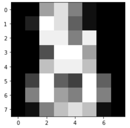
fromsklearnimportdatasetsiris=datasets.load_iris()digits=datasets.load_digits()# digits.data.shape, (1797, 64)# digits.images.shape, (1797, 8, 8)importmatplotlib.pyplotaspltplt.imshow(digits.images[-1],cmap='gray')fromsklearnimportsvm# first, we treat the estimator as a black box, and set params manually# or we can use `grid search` and `cross validation` to determine the best paramsclf=svm.SVC(gamma=0.001,C=100.)# train(or learn) from all (except last one) digits# validate with the last digitclf.fit(digits.data[:-1],digits.target[:-1])clf.predict(digits.data[-1:])
array([8])
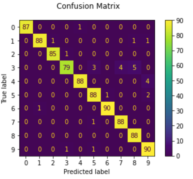
# better practisefromsklearn.model_selectionimporttrain_test_split# flatten the imagesn_samples=len(digits.images)data=digits.images.reshape((n_samples,-1))# Create a classifier: a support vector classifierclf=svm.SVC(gamma=0.001)# Split data into 50% train and 50% test subsetsX_train,X_test,y_train,y_test=train_test_split(data,digits.target,test_size=0.5,shuffle=False)# Learn the digits on the train subsetclf.fit(X_train,y_train)# Predict the value of the digit on the test subsetpredicted=clf.predict(X_test)
the example above, the float32 X is casst to float64 by fit_transform(X)
fromsklearnimportdatasetsfromsklearn.svmimportSVCiris=datasets.load_iris()clf=SVC()clf.fit(iris.data,iris.target)print(list(clf.predict(iris.data[:3])))# fit stringclf.fit(iris.data,iris.target_names[iris.target])print(list(clf.predict(iris.data[:3])))# ['setosa', 'setosa', 'setosa']
[0, 0, 0]
['setosa', 'setosa', 'setosa']
Refitting and updating parameters
Hyper-parameters of an estimator can be updated after it has been constructed via the set_params(). then you call fit(), the learned will be overwrite.
import numpy as np
from sklearn import datasets
iris_X, iris_y = datasets.load_iris(return_X_y=True)
# Split iris data in train and test data
# A random permutation, to split the data randomly
np.random.seed(0)
indices = np.random.permutation(len(iris_X))
iris_X_train = iris_X[indices[:-10]]
iris_y_train = iris_y[indices[:-10]]
iris_X_test = iris_X[indices[-10:]]
iris_y_test = iris_y[indices[-10:]]
# Create and fit a nearest-neighbor classifier
from sklearn.neighbors import KNeighborsClassifier
knn = KNeighborsClassifier()
knn.fit(iris_X_train, iris_y_train)
print(knn.predict(iris_X_test))
print(iris_y_test)
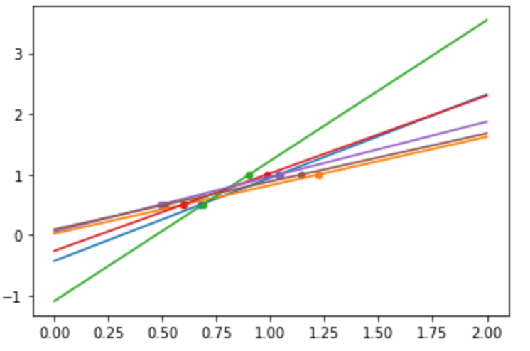
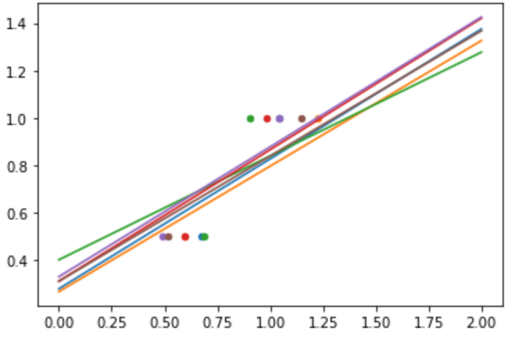
A solution in high-dimensional statistical learning is to shrink the regression coefficients to zero: any two randomly chosen set of observations are likely to be uncorrelated. This is called Ridge regression.
This is an example of bias/variance tradeoff:
the larger the ridge alpha parameter,
the higher the bias
the lower the variance.
lasso 回归和岭回归(ridge regression)其实就是在标准线性回归的基础上分别加入 L1 和 L2 正则化(regularization)。相比直接把一些特征的系数置零,只是把它们的“贡献”变小,即乘一下较低的权重(惩罚,imposing a penalty on the size of the coefficients)。
diabetes_X,diabetes_y=datasets.load_diabetes(return_X_y=True)diabetes_X_train=diabetes_X[:-20]diabetes_X_test=diabetes_X[-20:]diabetes_y_train=diabetes_y[:-20]diabetes_y_test=diabetes_y[-20:]# observe the alpha and the score:alphas=np.logspace(-4,-1,6)# log10(-4)到log10(-1)共6个数做alphaprint(alphas)print([f'{regr.set_params(alpha=alpha).fit(diabetes_X_train,diabetes_y_train).score(diabetes_X_test,diabetes_y_test)*100:.2f}%'foralphainalphas])
Different algorithms can be used to solve the same mathematical problem. For instance the Lasso object in scikit-learn solves the lasso regression problem using a coordinate descent method, that is efficient on large datasets. However, scikit-learn also provides the LassoLars object using the LARS algorithm, which is very efficient for problems in which the weight vector estimated is very sparse (i.e. problems with very few observations).
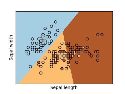
Classes are not always linearly separable in feature space. The solution is to build a decision function that is not linear but may be polynomial instead.
This is done using the kernel trick that can be seen as creating a decision energy by positioning kernels on observations:
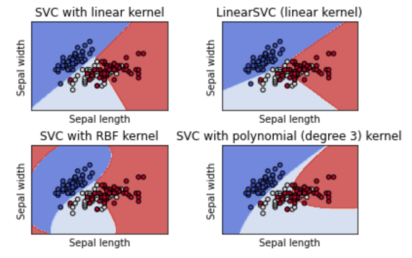
Linear kernal
svc=svm.SVC(kernel='linear')
Polynomial kernel
svc=svm.SVC(kernel='poly',degree=3)
RBF kernel (Radial Basis Function)
svc=svm.SVC(kernel='rfb')
DEMO: Plot different SVM classifiers in the iris dataset
LinearSVC minimizes the squared hinge loss while SVC minimizes the regular hinge loss.
LinearSVC uses the One-vs-All (also known as One-vs-Rest) multiclass reduction while SVC uses the One-vs-One multiclass reduction.
importnumpyasnpfromsklearnimportdatasets,svmX_digits,y_digits=datasets.load_digits(return_X_y=True)svc=svm.SVC(C=1,kernel='linear')score=svc.fit(X_digits[:-100],y_digits[:-100]).score(X_digits[-100:],y_digits[-100:])print(score)X_folds=np.array_split(X_digits,3)# 分成了3个foldy_folds=np.array_split(y_digits,3)scores=list()forkinrange(3):# We use 'list' to copy, in order to 'pop' later onX_train=list(X_folds)X_test=X_train.pop(k)# 取出最后一个fold # 不对,python居然可以Pop任意一个索引X_train=np.concatenate(X_train)# 把剩下的fold拼回去y_train=list(y_folds)y_test=y_train.pop(k)y_train=np.concatenate(y_train)scores.append(svc.fit(X_train,y_train).score(X_test,y_test))scores
对不同参数进行组合遍历,目的是为了maximize the cross-validation score
fromsklearn.model_selectionimportGridSearchCV,cross_val_scoreCs=np.logspace(-6,-1,10)clf=GridSearchCV(estimator=svc,param_grid=dict(C=Cs),n_jobs=-1)clf.fit(X_digits[:1000],y_digits[:1000])print('best score:',clf.best_score_)print('best estimator.c:',clf.best_estimator_.C)# Prediction performance on test set is not as good as on train setscore=clf.score(X_digits[1000:],y_digits[1000:])print('score:',score)
best score: 0.95
best estimator.c: 0.0021544346900318843
score: 0.946047678795483
与此同时,每个estimator也有自己的CV版本(跟之前串课的笔记呼应上了)
fromsklearnimportlinear_model,datasetslasso=linear_model.LassoCV()X_diabetes,y_diabetes=datasets.load_diabetes(return_X_y=True)lasso.fit(X_diabetes,y_diabetes)# The estimator chose automatically its lambda:lasso.alpha_
0.003753767152692203
Unsupervised learning: seeking representations of the data
$e(x) = \frac{1}{2}(f(x) - Y)^2$ (1/2的作用仅仅是为了取导数时消除常数项,简化计算)
$e'(x) = (f(x) - Y) \cdot f'(x) = \Delta y \cdot f'(x)\quad \color{green}{\Leftarrow Chain\ Rule}$
$\Delta x = e'(x) \cdot lr = \Delta y \cdot f'(x) \cdot lr\ \color{red}{\Leftarrow这里得到了更新x的依据}$
$x_{n+1} = x_n - \Delta x = x_n - \Delta y \cdot f'(x) \cdot lr \Leftarrow 公式有了$
这时可以写代码了
defgradient_sqrt(n):x=n/2# first trylr=0.01# learning rateepsilon=1e-10# quit flagf_x=lambdaa:a**2df_dx=lambdaa:2*adelta_y=lambdaa:f_x(a)-ne_x=lambdaa:delta_y(a)**2*0.5# funcon of lossde_dx=lambdaa:delta_y(a)*df_dx(a)# derivative of lossdelta_x=lambdaa:de_dx(a)*lrcount=0whileabs(x**2-n)>epsilon:count+=1x=x-delta_x(x)returnx,countforiinrange(1,10):print(f'sqrt({i}): {gradient_sqrt(i)}次')
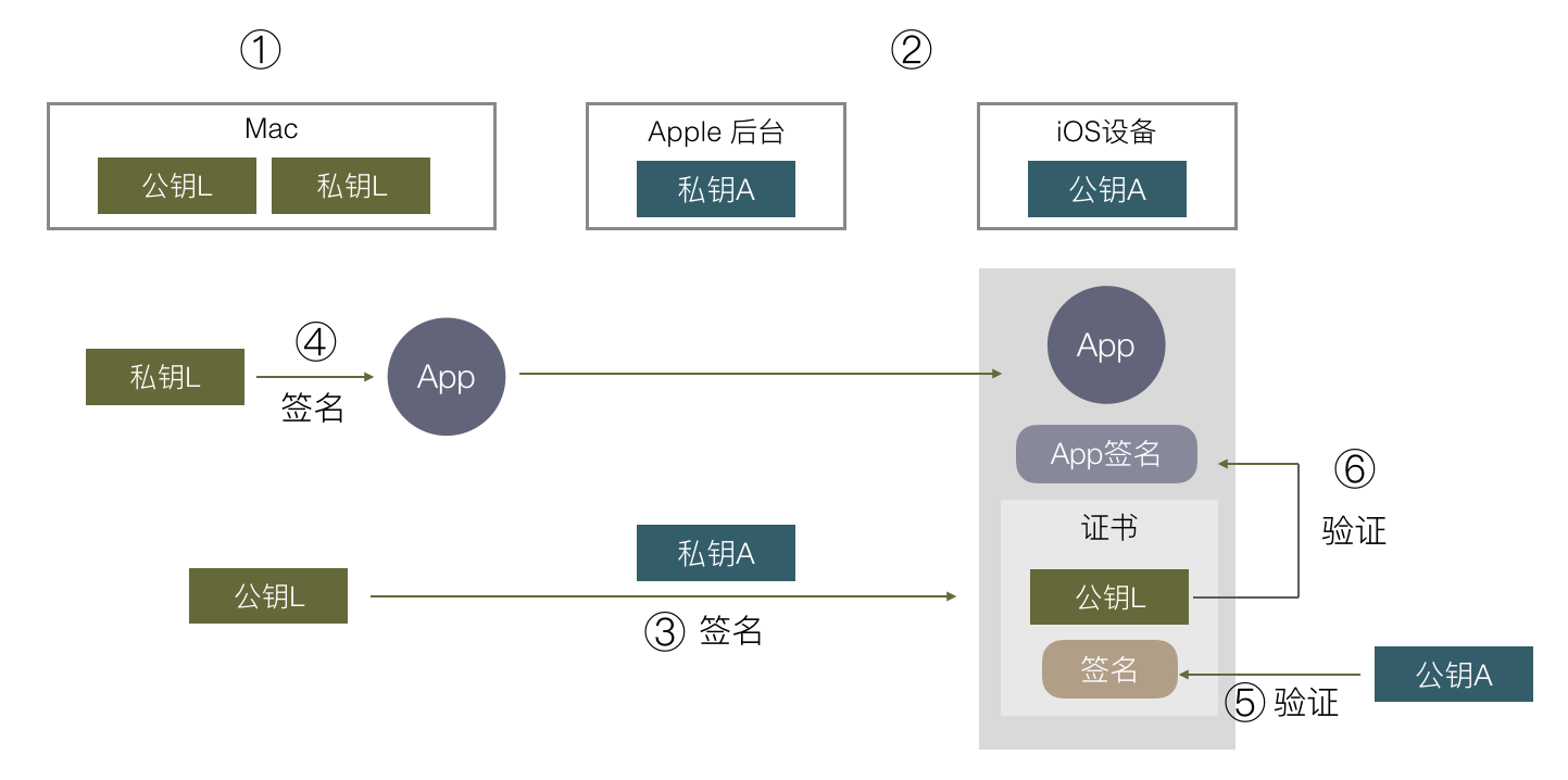
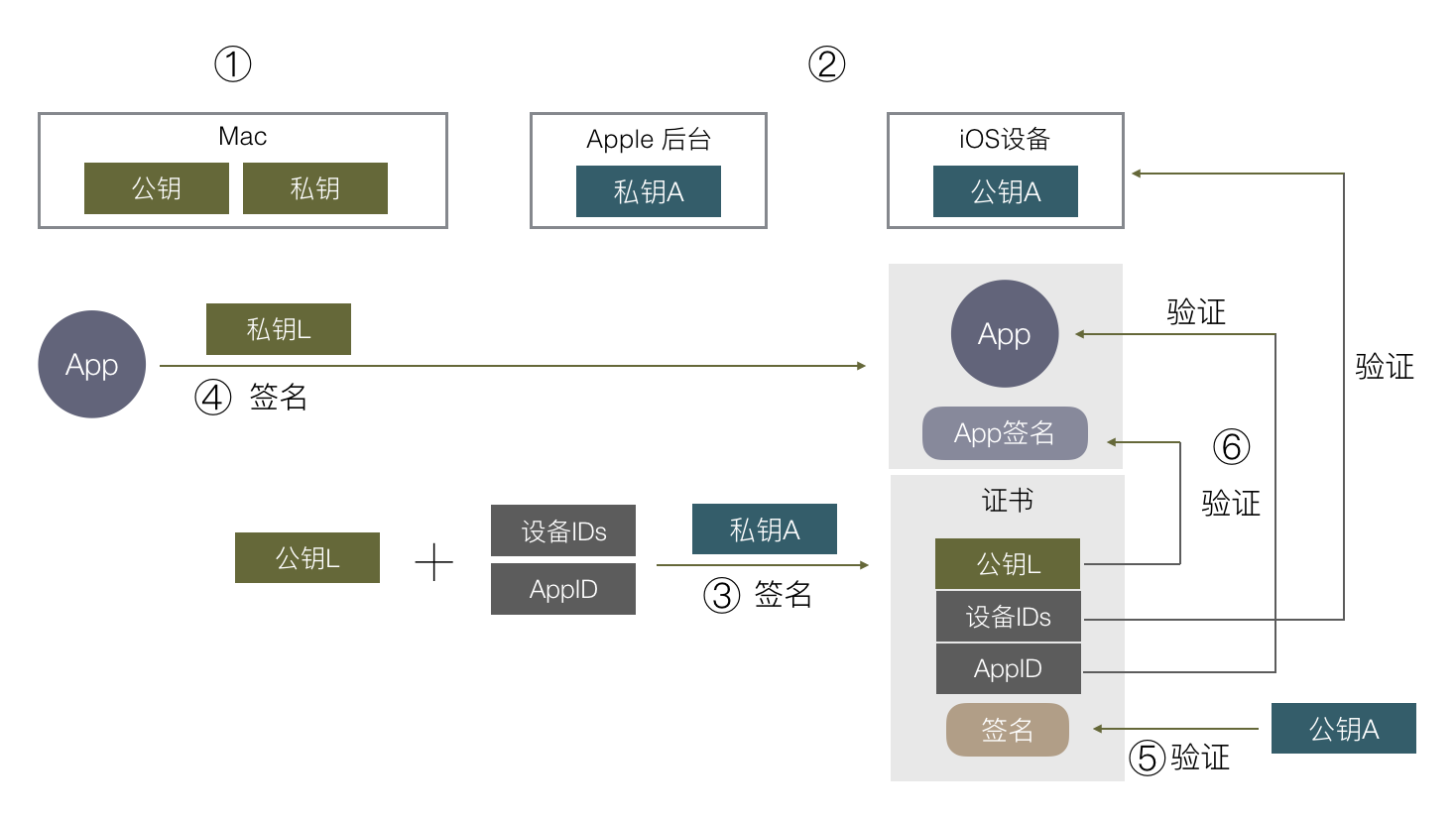
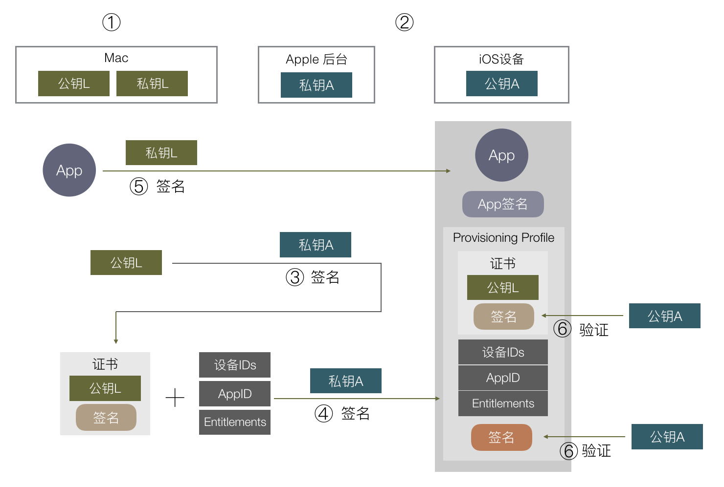
iOS 签名机制挺复杂,各种证书,Provisioning Profile,entitlements,CertificateSigningRequest,p12,AppID,概念一堆,也很容易出错,本文尝试从原理出发,一步步推出为什么会有这么多概念,希望能有助于理解 iOS App 签名的原理和流程。
https://wereadteam.github.io/2017/03/13/Signature/#%E7%9B%AE%E7%9A%84目的
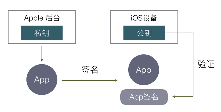
先来看看苹果的签名机制是为了做什么。在 iOS 出来之前,在主流操作系统(Mac/Windows/Linux)上开发和运行软件是不需要签名的,软件随便从哪里下载都能运行,导致平台对第三方软件难以控制,盗版流行。苹果希望解决这样的问题,在 iOS 平台对第三方 APP 有绝对的控制权,一定要保证每一个安装到 iOS 上的 APP 都是经过苹果官方允许的,怎样保证呢?就是通过签名机制。
https://wereadteam.github.io/2017/03/13/Signature/#%E9%9D%9E%E5%AF%B9%E7%A7%B0%E5%8A%A0%E5%AF%86非对称加密
通常我们说的签名就是数字签名,它是基于非对称加密算法实现的。对称加密是通过同一份密钥加密和解密数据,而非对称加密则有两份密钥,分别是公钥和私钥,用公钥加密的数据,要用私钥才能解密,用私钥加密的数据,要用公钥才能解密。
简单说一下常用的非对称加密算法 RSA 的数学原理,理解简单的数学原理,就可以理解非对称加密是怎么做到的,为什么会是安全的:
选两个质数 p
和 q
,相乘得出一个大整数n
,例如 p=61,q=53,n=pq=3233
选 1-n 间的随便一个质数 e
,例如 e = 17
经过一系列数学公式,算出一个数字 d
,满足:a. 通过 n
和 e
这两个数据一组数据进行数学运算后,可以通过 n 和 d 去反解运算,反过来也可以。b. 如果只知道 n
和 e
,要推导出 d
,需要知道 p
和 q
,也就是要需要把 n 因数分解。
上述的 (n,e)
这两个数据在一起就是公钥,(n,d)
这两个数据就是私钥,满足用公钥加密,私钥解密,或反过来公钥加密,私钥解密,也满足在只暴露公钥(只知道 n
和 e)的情况下,要推导出私钥 (n,d)
,需要把大整数 n
因数分解。目前因数分解只能靠暴力穷举,而n数字越大,越难以用穷举计算出因数 p
和 q
,也就越安全,当 n
大到二进制 1024 位或 2048 位时,以目前技术要破解几乎不可能,所以非常安全。
若对数字 d
是怎样计算出来的感兴趣,可以详读这两篇文章:RSA 算法原理(一)(二)https://wereadteam.github.io/2017/03/13/Signature/#%E6%95%B0%E5%AD%97%E7%AD%BE%E5%90%8D数字签名
现在知道了有非对称加密这东西,那数字签名是怎么回事呢?
数字签名的作用是我对某一份数据打个标记,表示我认可了这份数据(签了个名),然后我发送给其他人,其他人可以知道这份数据是经过我认证的,数据没有被篡改过。
有了上述非对称加密算法,就可以实现这个需求:
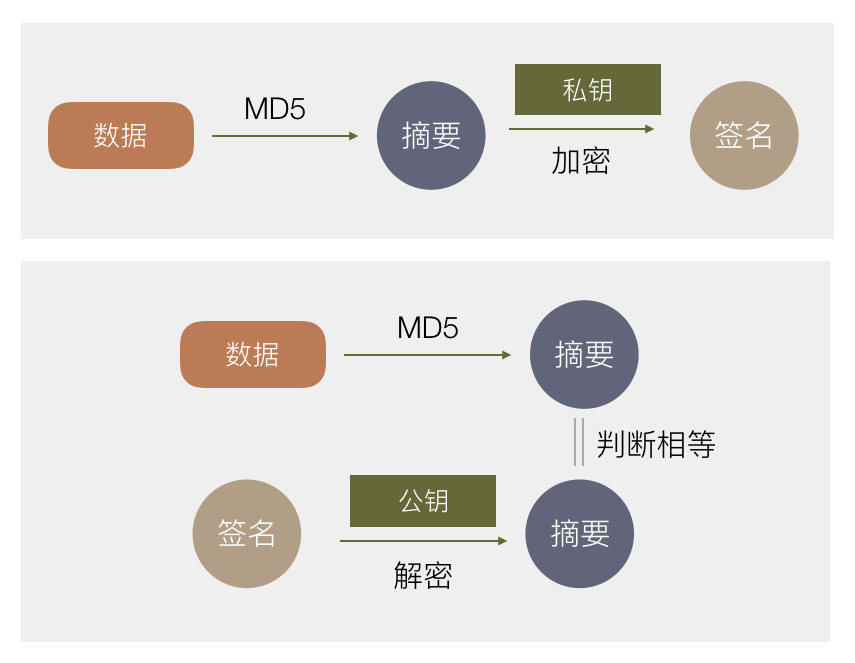
首先用一种算法,算出原始数据的摘要。需满足 a.若原始数据有任何变化,计算出来的摘要值都会变化。 b.摘要要够短。这里最常用的算法是MD5。
生成一份非对称加密的公钥和私钥,私钥我自己拿着,公钥公布出去。
对一份数据,算出摘要后,用私钥加密这个摘要,得到一份加密后的数据,称为原始数据的签名。把它跟原始数据一起发送给用户。
用户收到数据和签名后,用公钥解密得到摘要。同时用户用同样的算法计算原始数据的摘要,对比这里计算出来的摘要和用公钥解密签名得到的摘要是否相等,若相等则表示这份数据中途没有被篡改过,因为如果篡改过,摘要会变化。